Xuan Zhou*
Video Expression Recognition Method Based on Spatiotemporal Recurrent Neural Network and Feature Fusion
Abstract: Automatically recognizing facial expressions in video sequences is a challenging task because there is little direct correlation between facial features and subjective emotions in video. To overcome the problem, a video facial expression recognition method using spatiotemporal recurrent neural network and feature fusion is proposed. Firstly, the video is preprocessed. Then, the double-layer cascade structure is used to detect a face in a video image. In addition, two deep convolutional neural networks are used to extract the time-domain and airspace facial features in the video. The spatial convolutional neural network is used to extract the spatial information features from each frame of the static expression images in the video. The temporal convolutional neural network is used to extract the dynamic information features from the optical flow information from multiple frames of expression images in the video. A multiplication fusion is performed with the spatiotemporal features learned by the two deep convolutional neural networks. Finally, the fused features are input to the support vector machine to realize the facial expression classification task. The experimental results on cNTERFACE, RML, and AFEW6.0 datasets show that the recognition rates obtained by the proposed method are as high as 88.67%, 70.32%, and 63.84%, respectively. Comparative experiments show that the proposed method obtains higher recognition accuracy than other recently reported methods.
Keywords: Double Layer Cascade Structure , Facial Expression Recognition , Feature Fusion , Image Detection , Spatiotemporal Recursive Neural Network
1. Introduction
Emotional communication is the most natural way of communication between people. Facial expressions, for example, contain rich emotional information which make them important for exchanging information between people. Facial expression recognition methods for video [1-5] automatically recognize the emotional state of faces. Facial expression recognition technology remains an active research area; it has wide application prospects in the fields of human-computer interaction, virtual reality, security monitoring, and identity authentication
According to the format of the input image, facial expression recognition systems can be divided into two categories: expression recognition systems based on video and expression recognition systems based on static image [6,7]. In the video expression recognition systems, the spatial characteristics based on a static image cannot achieve a good facial expression classification of the video, because the method does not consider the temporal dynamics of the expression [8-10].
To improve the accuracy and computational efficiency of video expression recognition, a novel method using a recursive fusion of a space-time convolutional neural network (RFSCNN) is proposed. The main innovations of the proposed method are summarized as follows:
A two-layer cascade structure is proposed. It iterates continuously through a gradient boosting regression tree, which improves the convergence speed of the model and reduces errors.
Feature fusion is proposed. It integrates the learned spatiotemporal expression features and classifies them through the classifier, which improves the accuracy of the model.
The overall structure of the paper is as follows. The relevant work on video expression recognition and the motivation for the research problem are introduced in Section 2. Section 3 introduces the architecture and detailed process of the proposed method. The experimental verification on the video expression dataset and a comparative analysis with existing methods are presented in Section 4. The conclusions and prospects for future work are in Section 5.
2. Related Works
For the facial expression recognition of videos, scholars have proposed many methods. For example, the authors of [11] proposed a facial recognition method using differential geometric features, which improves model efficiency by extracting features with greater importance in the image. Sun et al. [12] proposed a facial expression recognition method combining kernel cooperative representation and deep subspace learning. The principal components analysis network and linear discriminant analysis network were used to better extract advanced features and represent the abstract semantics of the given data. Then, the features were mapped into the kernel space to capture their nonlinear similarity, which improved the accuracy of the model. Moeini et al. [13] proposed an expression recognition method based on dual dictionaries. By learning a regression dictionary and a feature dictionary, the real value was adjusted according to the probability of a given facial expression of the input image; this improved the accuracy of the model. Owusu et al. [14] proposed an expression recognition method based on multi-layer feed-forward neural networks and Haar features. It extracted the salient features of the face to improve the efficiency of the model. Jain et al. [15] proposed a hybrid deep convolutional neural network facial expression recognition method. The internal relationship of the image and the recursive network was extracted, and the time dependence of the image was considered in the classification process. This improved the accuracy rate of the model. However, these methods did not consider the edge features of the image.
The authors of [16] proposed the pattern averaging method to reduce the image dimension by averaging adjacent pixels, which reduced the model running time. Hossain and Yousuf [17] proposed a non-verbal communication real-time facial expression recognition system, which detected all face features through the OpenCV Haar Feature cascade classifier and improved the recognition rate of the model. Yuan and Mao [18] proposed exponential elastic preserving projections, which improved the recognition rate by extracting the local geometric and global information of the dataset through elastic preserving projections. Chen et al. [19] proposed a face expression recognition method based on the improved deep residual network. By using the ReLu activation function, the anti-noise capability and the recognition rate of the model were improved. Khan [20] proposed the facial expression recognition method based on the face feature detection and feature extraction of neural network. The Sobel horizontal edge detection method was used to reduce image noise points and improve the recognition rate of the model. However, when the amount of data was large, these methods were prone to overfitting.
Huang et al. [21] proposed a facial expression recognition method based on expression-targeted feature learning (ETFL), which improved the performance of the model by reducing intra-class variation and expanding inter-class differences. Liu et al. [22] proposed the self-adaptive metric learning video expression recognition method based on deep neural network. The adaptive cluster loss function was used to balance the differences of intra-class and inter-class variances, which improved the accuracy of the model. However, when the dataset was small, these methods were not effective.
Li et al. [23] proposed a new deep fusion convolutional neural network facial expression recognition method, which improved the recognition rate of the model by fusing all of the texture features in the image dataset. Yu et al. [24] proposed a deep cascaded peak-piloted network (DCPN), which extracted key and subtle details of the image through peak-lead feature transformation; this improved the recognition rate of the model. However, the running time of these methods was longer.
Boughrara et al. [25] proposed a multi-layer perceptron algorithm suitable for facial expression recognition, which increased the accuracy of the model by adding hidden neurons. However, the parameters were more difficult to adjust.
It can be seen from the above analysis that deep learning provides good modeling and processing capabilities for massive datasets [26,27]. Most existing facial expression recognition methods only consider spatial features and ignore the time-domain features, which limits their performance. To make full use of the time domain features in video expressions, the paper studies video expression recognition methods based on deep convolutional neural networks. The method consists of two aspects. One aspect is to extract high-level spatial and temporal features from the video, and the other is to fuse spatial and temporal features.
3. The Overall Architecture and Basic Concepts of the Proposed Method
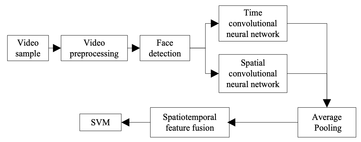
The proposed face expression recognition framework model using a spatiotemporal recurrent neural network and feature fusion is shown in Fig. 1. Two of its main components are the temporal and spatial convolutional neural networks. The time convolutional neural network processes the optical flow signal of the video and extracts the high-level temporal features. The spatial convolutional neural network processes the face image of each frame in the video and extracts the high-level spatial features. Then, an average pooling is performed on the extracted temporal and spatial features, and the spatial-temporal feature fusion based on a DBN is performed on the feature layer. Finally, the support vector machine (SVM) is used to complete the classification task of the video expressions. The model mainly includes three steps: video preprocessing, deep space-time expression feature extraction, and fusion expression classification.
3.1 Video Preprocessing
The duration of each video is different; however, the [TeX:] $$D C N N_{S}$$ needs a fixed size of data input. Therefore, in the paper, the video is divided into many segments of a fixed duration, which are used as the input to the time and spatial convolutional neural networks. In this way, the dataset for the [TeX:] $$D C N N_{S}$$ training can also be expanded to a certain extent.
Assume L represents the number of frames contained in the video clip. It is also important to select the appropriate size L for the extraction of time information features of the video. If L is too small, the video segment contains insufficient dynamic change information. Conversely, if it is too large, the video clip may contain excessive noise, which affects the recognition performance.
In the paper, by searching L in the range of [2,20], we find that when L=16, the time convolutional neural network achieves the best effect. Therefore, this paper divides each video into 16-frame fragments. When [TeX:] $$L>16$$, the preceding and following [TeX:] $$(L-16) / 2$$ frames of the video are discarded. When [TeX:] $$L<16$$, the preceding and following [TeX:] $$(16-L) / 2$$ frames of the video are copied. For a video segment with L=16, it contains 15 frames of optical flow images, because every two adjacent spatial images generate a one frame optical flow image. The optical flow image represents the displacement information of the corresponding positions for the two adjacent frames. The specific calculation process is as follows. Suppose the two adjacent frames in the video are t and t+1, and the displacement vector [TeX:] $$d_{t}$$ represents the displacement information of the video. The optical flow image [TeX:] $$I_{t}$$ is composed of [TeX:] $$d_{t} x \text { and } d_{t} y$$. The two channels of [TeX:] $$I_{t} \text { are } d_{t} x \text { and } d_{t} y$$. These represent the horizontal and the vertical displacement component of the position of two adjacent frames in the video, respectively. The input of the [TeX:] $$D C N N_{S}$$ is the RGB image with three channels. Therefore, the amplitude component [TeX:] $$d t_{z}$$ of the optical flow image [TeX:] $$I_{t}$$ is calculated as the third channel of [TeX:] $$I_{t}$$.
For the preprocessing of the input image of the spatial convolutional neural network, the face image contained in each frame of the video clip is extracted in real time. The size of the area containing the key expression parts such as mouth, nose, forehead from the original face image is an image with the size of 150×110×3. The image is the input of the spatial convolutional neural network. The extracted optical flow image and facial expression image are scaled to 227×227×3.
3.2 Face Detection
Due to large image differences and rough initializations, the single-layer regressor [28] is not suitable for the entire model. The main reasons are: the single regressor is too weak, the convergence is slow during training, and the results are poor during testing. To converge faster and be more stable during training, a double-layer cascade structure is used as shown in Fig. 2.
Firstly, there is a training set [TeX:] $$\left(I_{1}, S_{1}\right), \ldots\left(I_{i}, S_{i}\right), \text { where } I_{i}$$ is a picture and [TeX:] $$S_{i}$$ is the position of key points of the face. In the regression training of the first layer, the training dataset can be written as [TeX:] $$\left(I_{i}, \hat{S}_{i}^{(t)}, \Delta S_{i}^{(t)}\right)$$, where [TeX:] $$I_{i}$$ is the picture of the dataset and [TeX:] $$\hat{S}_{i}^{(t)}$$ is the predicted key point position of the t layer of the first layer cascade regression. [TeX:] $$\Delta S_{i}^{(t)}$$ is the difference between the regression result and the true value of the layer. Its iteration formula is:
When the first layer of regression cascade layers is set to T layers, the regressors [TeX:] $$r_{1}, r_{2}, \cdots r_{T}$$ are generated. These T regressors are the regression model required by training.
The second layer trains each regressor [TeX:] $$r_{t}$$ The way to build the regressor in this paper is to use gradient boosted regression trees. Each regressor uses a square error function to fit the residuals. The residuals calculated in each tree correspond to the gradient of the loss function evaluated by each training sample.
Since a regression tree is a weak regressor, both the feature indexing method and the splitting principle are simple approaches; the regression results have limited accuracy. To improve the accuracy, a weight value (less than one) is added to the regression result of each decision tree. More specifically, for each base learner [TeX:] $$g_{k}$$, a reduction factor v is set and the weight is added in the accumulation step. The regression goal of the regression tree remains the residual. The regression of each tree to the residual is a relatively smooth process and has no mutation; these beneficial characteristics are due to the use of a set of relatively small step sizes. However, adding the reduction factor slows down the training speed of the regressor.
3.3 Spatiotemporal Recurrent Neural Network
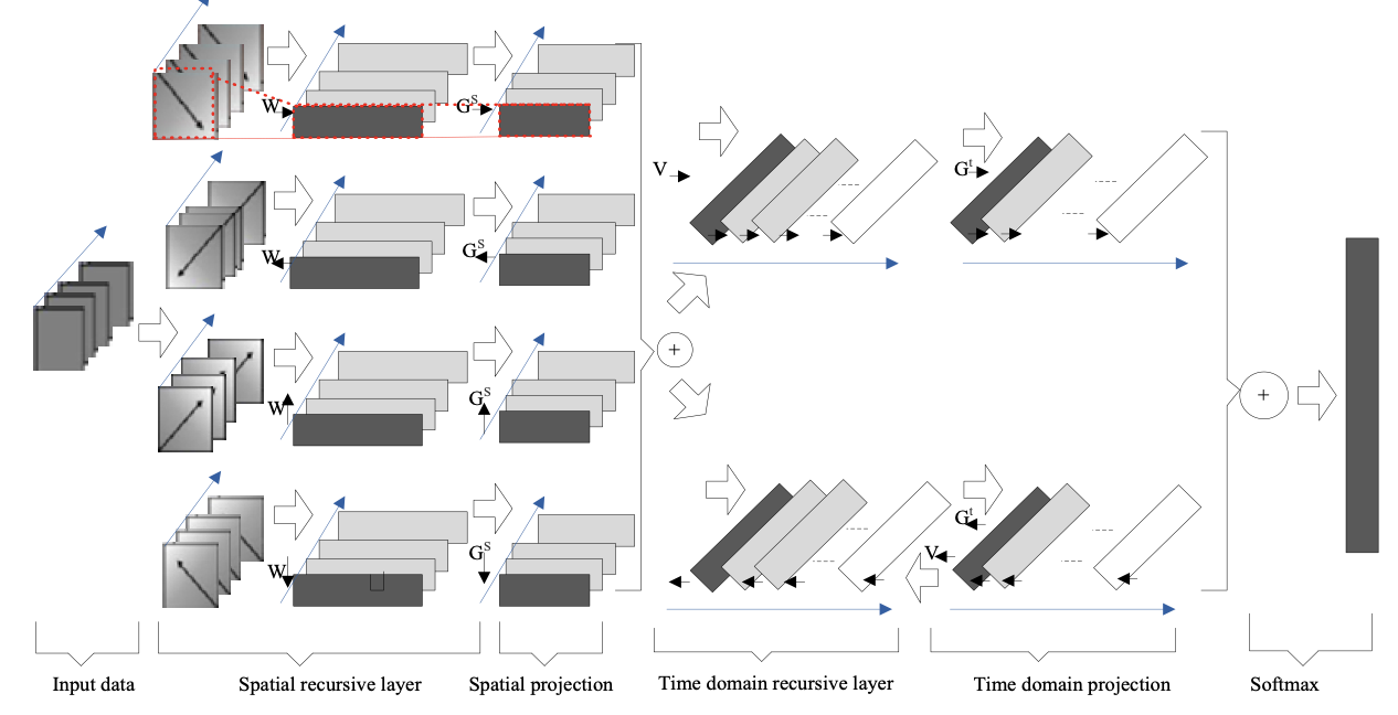
The input of the RFSCNN can be any data with spatiotemporal structure [29], including a multi-channel signal sequence or a spatiotemporal cube. Because the video sequence is a spatially regular grid structure, the entire network structure includes three layers: spatial recursion layer, time domain recursion layer, and softmax classification layer. The basic framework of the RFSCNN is illustrated in Fig. 3.
The RFSCNN captures spatiotemporal information with a high discriminant in emotional signals. To achieve this, the model stacks a spatial recursive layer and a temporal recursive layer. These are connected with other network layers to form a whole. Both the spatial and the temporal recursive layers contain multiple features in space or time. For each feature, the hidden state generated at the previous moment is passed to the current moment. This hidden state is used with the current input to calculate the hidden state at the next moment. The recursive learning process makes the convolutional layer present a deep structure, which can better learn the correlation between the states in the sequence and establish the long-term correlation between the regions. In addition, the benefits of the RFSCNN are that the spatial recursive layer and the temporal recursive layer can be used as two memory units to memorize and encode all of the scanned spatial and temporal regions. This approach can globally optimize and learn the spatial and temporal related information in the emotional data.
To better model the spatial correlation of each time slice in sentiment data, the spatial recursive layer first stretches and transforms the data exhibiting a two-dimensional spatial layout into a one-dimensional sequence. Then, the sequence is scanned in a predetermined order. As a result, the operation process is simplified by expanding the two-dimensional spatial structure into an ordered one-dimensional sequence. This makes the learning process more efficient and controllable. After scanning the elements sequentially on each time slice, the convolutional layer can better characterize the high-level semantic information and inter-region related information contained between them. It is worth noting that emotion data usually contain interference information. Here, the spatial recursive layer uses four convolutional layers that scan in different directions to traverse each time slice from four specific angles. Since the four convolutional layers are complementary in direction, they can construct a complete spatial relationship and the robustness of the model is also enhanced. The spatial domain recursive layer represents the t time slice (represented as [TeX:] $$X_{t}$$) as a graph when modeling the spatial correlation. The graph is denoted as [TeX:] $$g_{t}=\left\{R_{t}, C_{t}\right\}$$. Each spatial element in [TeX:] $$X_{t}$$ can be used as a vertex of the graph [TeX:] $$g_{t}$$. [TeX:] $$R_{t}=\left\{x_{t i j}\right\}(i=1, \ldots h, j=1, \ldots, w)$$ represents a set of vertices composed of all vertices. i and represent the spatial position of each vertex element. [TeX:] $$c_{t}=\left\{e_{t i j, t k l}\right\}$$ represents the edge composed of spatially adjacent elements in [TeX:] $$X_{t}$$. Based on the constructed graph [TeX:] $$g_{t}$$, the spatial recursive layer traverses the vertices in the graph in a predefined order. The traversal method also defines the current input state and the previous state for the neural unit. Therefore, the spatial recursive layer can be defined as follows:
(4)
[TeX:] $$h_{t i j}^{r}=\sigma_{1}\left(U^{r} X_{t i j}+\sum_{k=1}^{h} \sum_{l=1}^{w} W^{r} h_{t k l}^{r} \times e_{t i j, t k l}+b^{r}\right)$$
(5)
[TeX:] $$e_{t i j, t k l}=\left\{\begin{array}{l} 1, i f(k, l) \in \mathrm{N}_{i j}^{r} \\ 0, \text { other } \end{array}\right.$$Among them, [TeX:] $$X_{t i j} \text { and } h_{t i j}^{r}$$ represent the input node and the hidden node at the position of and in the t time slice, respectively. According to the above process, the spatial recursive layer traverses the correlation between the time and spatial dimensions in four different directions to model and learn the emotional features with high discriminability.
In the process of traversing all of the vertices of [TeX:] $$R_{t}$$ in the spatial recursive layer, the number of hidden states generated for each given traversal direction is equal to the number of elements on each time slice, h×w. The hidden state [TeX:] $$h_{t i j}^{r}(i=1, \ldots, h, j=1, \ldots, w)$$ is rewritten as [TeX:] $$h_{t k}^{r}(k=1, \ldots, K)$$, and K=h×w. To further detect the significant regions of emotional expression, the RFSCNN projects the hidden states generated in each traversal direction with sparse constraints. Assume that the projection matrix in a certain traversal direction is expressed by [TeX:] $$G^{r}=\left[G_{i j}^{r}\right]_{K \times K_{d}}$$, where [TeX:] $$K_{d}$$ represents the number of hidden states after projection. The sparse projection process can be expressed as follows:
After sparse projection, all the features of the temporal recursive layer can be integrated as:
where, [TeX:] $$P^{r}$$ is the optimizable projection matrix corresponding to each traversal direction.
In the temporal recursive layer, assume that the time length of the emotion sequence is L. When passing through the spatial recursive layer, the spatial features generated by each time slice are [TeX:] $$m_{t}, t=1, \ldots, L$$. Then, the forward and reverse learning process of the temporal recursive layer can be represented as follows:
[TeX:] $$\left\{R^{f}, V^{f}, b^{f}\right\} \text { and }\left\{R^{b}, V^{b}, b^{b}\right\}$$ are the optimizable parameters during the forward and reverse traversals, respectively. [TeX:] $$m_{t}, h_{t}^{f}, \text { and } h_{t}^{b}$$ are the hidden states generated by the input features and the bidirectional convolution layer, respectively. After sparse projection, the feature quantities output at time t of the bidirectional convolution layer can be expressed as:
(10)
[TeX:] $$\begin{array}{l} \mathrm{q}_{t}^{f}=\sum_{i=1}^{L} G_{i t}^{f} h_{i}^{f} \\ q_{t}^{b}=\sum_{i=1}^{L} G_{i t}^{b}, t=1, \cdots, L_{d} \end{array}$$[TeX:] $$G^{f}=\left[G_{i j}^{f}\right]_{L \times L_{d}} \text { and } G^{b}=\left[G_{i j}^{b}\right]_{L \times L_{d}}$$ represent the sparse projection matrix of [TeX:] $$h_{t}^{f}, h_{t}^{b} . L_{d}$$ represents the length of the sequence after the projection. These are integrated as:
where [TeX:] $$P^{f}$$ and [TeX:] $$P^{b}$$ are the optimizable projection matrices corresponding to [TeX:] $$P^{f}$$ and [TeX:] $$P^{b}$$ respectively. [TeX:] $$o=\left[o_{1}, o_{2}, \cdots o_{C}\right]^{T}$$ is the output of the temporal recursive layer. C represents the number of sentiment categories.
3.4 Spatiotemporal Feature Fusion
The function completed by the fusion layer [30] is to fuse multiple networks at its output layer to form a network. There are three ways to accomplish the fusion including connection, summation, and quadrature. Assume that the two networks have output vectors of the same dimension, which are [TeX:] $$x=\left(x_{1}, x_{2}, \cdots, x_{n}\right) \text { and } y=\left(y_{1}, y_{2}, \cdots, y_{n}\right)$$, respectively. The fusion layer fuses them into a vector using the following method.
Connection method: two vectors are spliced, and the splicing formula is as follows:
Summing method: add the two vectors by element, and the summation formula is as follows:
Quadrature method: multiply the two vectors by elements, and the quadrature formula is as follows:
(14)
[TeX:] $$m(x, y)=\left(x_{1} \times y_{1}, x_{2} \times y_{2}, \cdots, x_{n} \times y_{n}\right)$$3.5 Loss Function
In the task of facial expression recognition, the input of the neural network is convolved, activated, and pooled. Its output is pulled into a vector to enter several fully connected layers. The number of fully connected neurons in the last layer is the same as the number of sample categories. The probability that the sample belongs to each category is obtained through the softmax function. Assume that the category number of samples is c and the output of the last fully connected layer is [TeX:] $$z \in R^{C}$$. Then, the probability that the output sample z_i of the i neuron to category after the softmax function is applied is:
For the classification task, the cross-entropy loss function is used. Assume that the true label of the sample is [TeX:] $$y \in R^{C}$$, expressed by a one-hot vector. The cross-entropy loss function is:
The denominator of each output of the softmax function contains [TeX:] $$Z_{i}$$. When calculating the partial derivative of L with respect to [TeX:] $$Z_{i}$$, it is necessary to consider the case where other elements are not [TeX:] $$Z_{i}$$. The chain rule yields:
(17)
[TeX:] $$\frac{\partial L}{\partial z_{i}}=\frac{\partial L}{\partial s_{j}} \cdot \frac{\partial s_{j}}{\partial z_{i}}$$The first term on the right side of Eq. (17) can obtain:
(18)
[TeX:] $$\frac{\partial L}{\partial z_{i}}=\frac{\partial\left(-\sum_{j=1}^{c} y_{j} \ln s_{j}\right)}{\partial s_{j}}=-\sum_{j=1}^{c} \frac{y_{j}}{s_{j}}$$The second term on the right side of Eq. (17) can obtain the following two cases: [TeX:] $$i=j \text { and } i \neq j$$:
(19)
[TeX:] $$\frac{\partial \mathbf{s}_{j}}{\partial z_{i}}=\frac{\frac{e^{z_{i}}}{\sum_{k=1}^{c} e^{z_{k}}}}{\partial z_{i}}, i=j$$
(20)
[TeX:] $$\frac{\partial \mathbf{s}_{j}}{\partial z_{i}}=\frac{\frac{e^{z_{j}}}{\sum_{k=1}^{c} e^{z_{k}}}}{\partial z_{i}}, i \neq j$$Eqs. (19) and (20) can be simplified to:
(21)
[TeX:] $$\frac{\partial \mathbf{s}_{j}}{\partial z_{i}}=\left\{\begin{array}{l} s_{i}\left(1-s_{i}\right), i=j \\ -s_{i s_{j}}, i \neq j \end{array}\right.$$Eqs. (18) and (21) are substituted into Eq. (17) to obtain:
(22)
[TeX:] $$\begin{aligned} \frac{\partial L}{\partial \mathbf{z}_{i}} &=-\frac{y_{i}}{s_{i}} s_{i}\left(1-s_{i}\right)+\sum_{j \neq i} \frac{y_{j}}{s_{j}} s_{i} s_{j} \\ &=-y_{i}+s_{i} \sum_{j=1}^{c} y_{j}=s_{i}-y_{i} \end{aligned}$$Thus, the overall architecture of the convolutional neural network can be obtained. The front end is composed of multiple layers of convolution, activation, and pooling. The back end obtains the final classification results through several fully connected layers. Therefore, the process including feature extraction, feature selection, and classifier learning, previously accomplished separately in the traditional methods, is completed end-to-end in the proposed approach.
4. Experimental Results and Analysis
To verify the effectiveness of the proposed video facial expression recognition method using spatiotemporal recursive neural network and feature fusion, experimental evaluations are performed on the cNTERFACE, RML, and AFEW6.0 datasets. A comparative study is presented using the ETFL [21], DCPN [24], and the proposed RFSCNN. These methods are implemented using Python3.0.
4.1 Experimental Dataset
The cNTERFACE dataset contains video samples of six basic emotion categories tested by 44 participants. Each subject has five samples under each expression. Due to the lack of samples or the problem of unsegmented video, a total of 1,287 video samples of 43 participants were available for the experiment.
The RML dataset has 720 videos and consists of eight people's expressions. There are six kinds of expressions on the dataset, including angry, hate, fear, happy, sadness, and surprise. The average duration of each video sample is approximately five seconds. The size of each image in the video is 720×480×3.
The AFEW6.0 dataset contains 773 training samples, 383 verification samples, and 593 test samples. The video clip samples are from Hollywood movies and reality TV shows.
4.2 Analysis of Parameter Performance
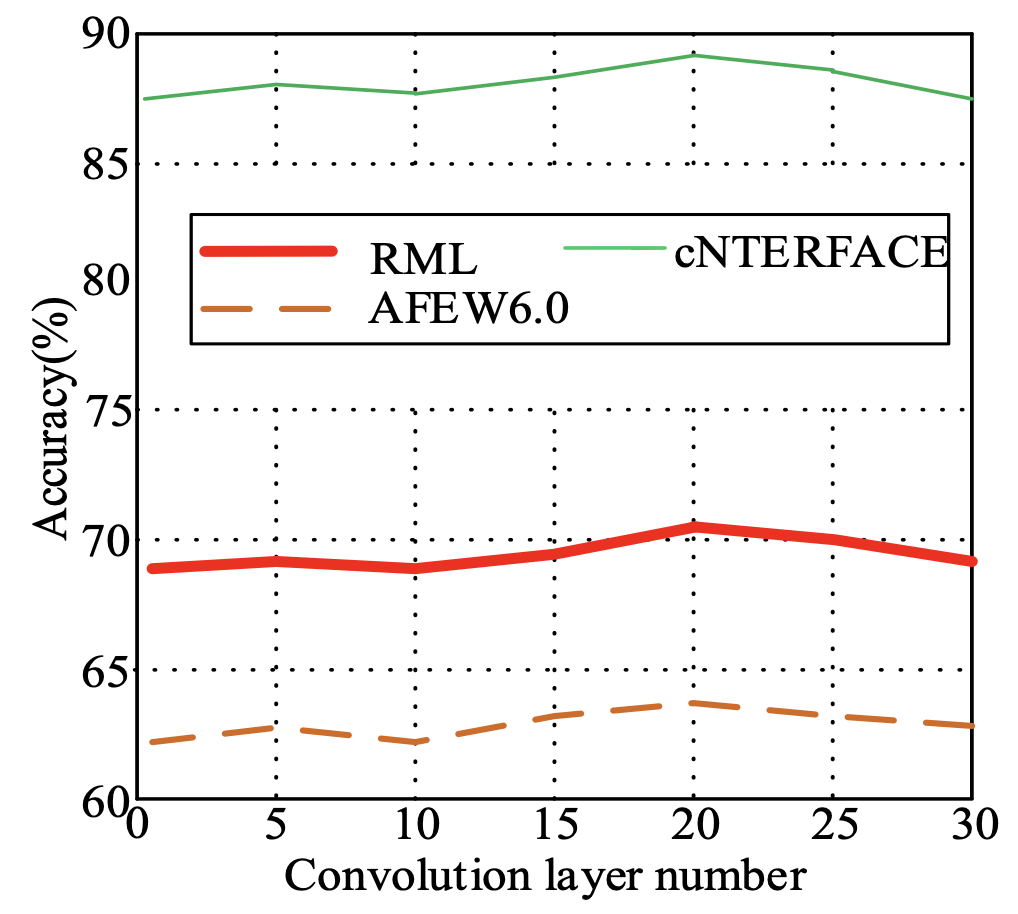
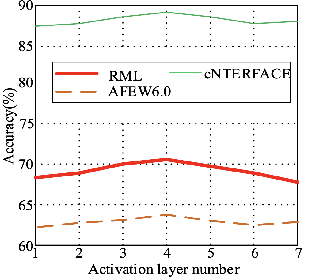
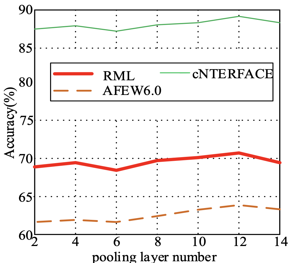
To verify the number of layers of convolution layer, activation layer, and pooling layer of the proposed video facial expression recognition method using the spatial-temporal recurrent neural network and feature fusion, experiments were carried out on the RML, cNTERFACE, and AFEW6.0 datasets. In the experiment, the number of convolutional layers varies from 1 to 35, the number of activation layers varies from 1 to 7, and the number of pooling layers varies from 2 to 14. The experimental results are shown in Figs. 4-6.
As can be seen from Figs. 4–6, when the number of convolutional layers is 20, the number of active layers is 4, and the number of pooling layers is 12, the model can extract spatiotemporal features with a strong characterization ability. The recognition rates on the RML, cNTERFACE, and AFEW6.0 datasets have reached the maximum. Therefore, in the following experiments, the numbers of convolutional layers, active layers, and pooling layers are set to 20, 4, and 12.
4.3 Feature Fusion Verification
For the convolutional layer, the number of the first layer is set to 8 and the number of the second layer is set to 16. The number of neurons of the fully connected layer is 64. Under the same feature extraction method, the experiment analyzes the differences of recognition rates for the temporal feature, spatial feature, and spatial fusion feature in the three datasets. The experimental results are shown in Table 1.
It can be seen from Table 1 that the recognition rates of the temporal and spatial features are slightly lower because the discriminative semantic features of the dataset have not been learned. The recognition rate of the spatial and temporal feature fusion method is slightly higher because the learned image features are more complete and more discriminative.
Table 1.
| Fusion method | Accuracy rate (%) | ||
|---|---|---|---|
| cNTERFACE | RML | AFEW6.0 | |
| Temporal feature | 71.35 | 58.33 | 51.36 |
| Spatial feature | 74.77 | 65.44 | 55.61 |
| Spatiotemporal features | 88.67 | 70.32 | 63.84 |
4.4 Recognition Results
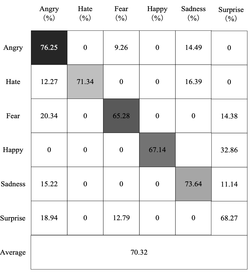
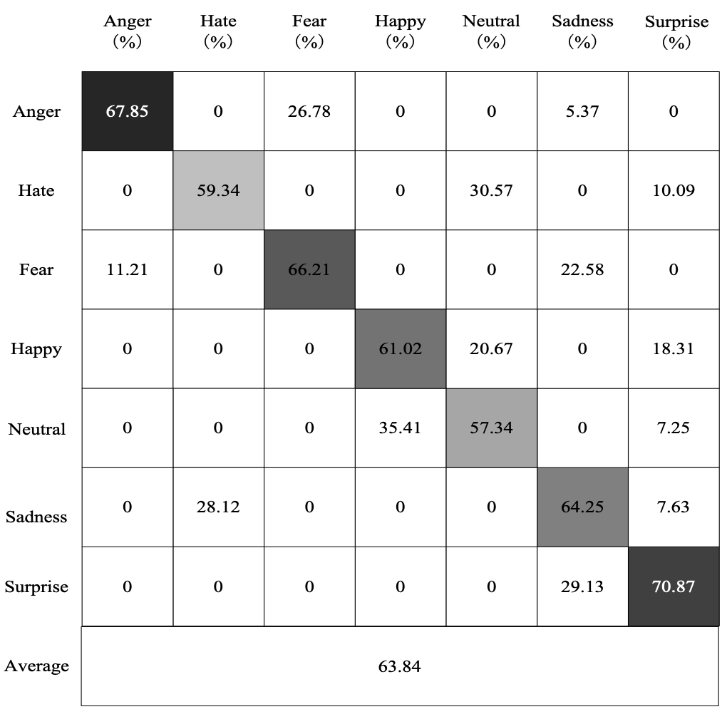
To illustrate the recognition of each expression by the proposed method, Figs. 7-9 show the confusion matrix when the RFSCNN achieves the best performance on the cNTERFACE, RML, and AFEW6.0 datasets.
It can be seen from Figs. 7-9 that the recognition effect on the cNTERFACE dataset is the best; the recognition rate is as high as 88.67%. In the RML dataset, fear is more difficult to identify. In the AFEW6.0 dataset, average is more difficult to identify. The correct recognition rates are 65.28% and 57.34% for fear and average in these two datasets, respectively. The reason is that the characteristics of the expression are similar with those of other expressions and are easily confused.
4.5 Comparison with Other Methods
The experiment shows the comparison between the proposed method and two existing methods on the cNTERFACE, RML and AFEW6.0 datasets. All comparisons are carried out using LOGO cross-validation. It is best to ensure that the training object is carried out under conditions independent of the test object. The classifier also uses an SVM. The experimental results are shown in Table 2.
Table 2.
| Database | ETFL (%) | DCPN (%) | RFSCNN (%) |
|---|---|---|---|
| cNTERFACE | 78.68 | 82.34 | 88.67 |
| RML | 62.06 | 65.81 | 70.32 |
| AFEW6.0 | 55.21 | 58.36 | 63.84 |
It can be seen from Table 2 that compared with two other existing methods, the recognition effect of the RFSCNN is optimal: the final expression recognition rate is improved by 8.26%-9.99%. Compared with traditional methods based on manual features, the RFSCNN is more suitable for facial expression recognition scenarios.
5. Conclusion and Future Work
In this paper, a new video facial expression recognition method using a spatiotemporal recursive neural network and feature fusion is proposed. The training process is divided into two stages. Firstly, the temporal and spatial convolutional neural networks are adjusted to extract more discriminative features from the dataset. Secondly, the learned temporal and spatial features are fused. The experimental results show that the training performed under the proposed RFSCNN network and the same classifier results in a superior expression recognition effect.
In the future, investigating the serialized facial expression recognition task is going to focus on reducing the complexity of the network structure and reducing the number of model parameters of the RFSCNN. These reductions seek to support the accurate and efficient analysis of sequences with a larger number of frames.
Biography
Xuan Zhou
https://orcid.org/0000-0002-2244-9218He earned his Master’s degree of Education, Engineer, Graduated from Hangzhou Normal University in 2012. He is a lecturer at Hangzhou Normal University Qianjiang College. He worked in Qianjiang College of Hangzhou Normal University, China. His research interests include information technology and multimedia technology.
References
- 1 J. Li, Y. Mi, G. Li, Z. Ju, "CNN-based facial expression recognition from annotated rgb-d images for human–robot interaction," International Journal of Humanoid Robotics2019, vol. 16, no. 4, 1941.doi:[[[10.1142/S021984360020]]]
- 2 M. U. Nagaral, T. H. Reddy, "Hybrid approach for facial expression recognition using HJDLBP and LBP histogram in video sequences," International Journal of ImageGraphics and Signal Processing, vol. 10, no. 2, pp. 1-9, 2018.doi:[[[10.5815/ijigsp..02.01]]]
- 3 X. Fan, X. Y ang, Q. Y e, Y. Y ang, "A discriminative dynamic framework for facial expression recognition in video sequences," Journal of Visual Communication and Image Representation, vol. 56, pp. 182-187, 2018.custom:[[[-]]]
- 4 F. Ahmed, M. H. Kabir, "Facial expression recognition under difficult conditions: a comprehensive study on edge directional texture patterns," International Journal of Applied Mathematics and Computer Science, vol. 28, no. 2, pp. 399-409, 2018.doi:[[[10.2478/amcs--0030]]]
- 5 H. Yan, "Collaborative discriminative multi-metric learning for facial expression recognition in video," Pattern Recognition, vol. 75, pp. 33-40, 2018.custom:[[[-]]]
- 6 J. Zhao, X. Mao, J. Zhang, "Learning deep facial expression features from image and optical flow sequences using 3D CNN," The Visual Computer, vol. 34, no. 10, pp. 1461-1475, 2018.custom:[[[-]]]
- 7 A. M. Shabat, J. R. Tapamo, "Angled local directional pattern for texture analysis with an application to facial expression recognition," IET Computer Vision, vol. 12, no. 5, pp. 603-608, 2018.custom:[[[-]]]
- 8 Z. Gong, H. Chen, "Sequential data classification by dynamic state warping," Knowledge and Information Systems, vol. 57, no. 3, pp. 545-570, 2018.custom:[[[-]]]
- 9 O. Yi, H. Tavafoghi, D. Teneketzis, "Dynamic games with asymmetric information: common information based perfect Bayesian equilibria and sequential decomposition," IEEE Transactions on Automatic Control, vol. 62, no. 1, pp. 222-237, 2016.custom:[[[-]]]
- 10 L. H. Nguyen, J. A. Goulet, "Real-time anomaly detection with Bayesian dynamic linear models," Structural Control and Health Monitoring, vol. 26, no. 9, 2019.doi:[[[10.1002/stc.2404]]]
- 11 E. Zangeneh, A. Moradi, "Facial expression recognition by using differential geometric features," The Imaging Science Journal, vol. 66, no. 8, pp. 463-470, 2018.doi:[[[10.1080/13682199..1509176]]]
- 12 Z. Sun, Z. P. Hu, R. Chiong, M. Wang, W. He, "Combining the kernel collaboration representation and deep subspace learning for facial expression recognition," Journal of CircuitsSystems and Computers, 2018, vol. 27, no. 8, 2181.doi:[[[10.1142/S026618501219]]]
- 13 A. Moeini, K. Faez, H. Moeini, A. M. Safai, "Facial expression recognition using dual dictionary learning," Journal of Visual Communication and Image Representation, vol. 45, pp. 20-33, 2017.custom:[[[-]]]
- 14 E. Owusu, J. D. Abdulai, Y. Zhan, "Face detection based on multilayer feed-forward neural network and Haar features," Software: Practice and Experience, vol. 49, no. 1, pp. 120-129, 2019.doi:[[[10.1002/spe.2646]]]
- 15 N. Jain, S. Kumar, A. Kumar, P. Shamsolmoali, M. Zareapoor, "Hybrid deep neural networks for face emotion recognition," Pattern Recognition Letters, vol. 115, pp. 101-106, 2018.custom:[[[-]]]
- 16 N. P. Gopalan, S. Bellamkonda, "Pattern averaging technique for facial expression recognition using support vector machines," IJ ImageGraphics and Signal Processing, 27-33, vol. 9, 2018.doi:[[[10.5815/ijigsp..09.04]]]
- 17 M. S. Hossain, M. A. Yousuf, "Real time facial expression recognition for nonverbal communication," International Arab Journal of Information Technology, vol. 15, no. 2, pp. 278-288, 2018.custom:[[[-]]]
- 18 S. Yuan, X. Mao, "Exponential elastic preserving projections for facial expression recognition," Neurocomputing, vol. 275, pp. 711-724, 2018.custom:[[[-]]]
- 19 Y. Chen, J. Du, Q. Liu, L. Zhang, Y. Zeng, Robust, energy-efficient expression recognition based on improved deep ResNets, " Biomedical Engineering/Biomedizinische Technik2019, vol. 64, no. 5, pp. 519-528, 2018.doi:[[[10.1515/bmt--0027]]]
- 20 F. Khan, 2018 (Online). Available:, https://arxiv.org/abs/1812.04510
- 21 Y. Huang, Y. Y an, S. Chen, H. Wang, "Expression-targeted feature learning for effective facial expression recognition," Journal of Visual Communication and Image Representation, vol. 55, pp. 677-687, 2018.custom:[[[-]]]
- 22 X. Liu, Y. Ge, C. Y ang, P. Jia, "Adaptive metric learning with deep neural networks for video-based facial expression recognition," Journal of Electronic Imaging, vol. 27, no. 1, 2008.doi:[[[10.1117/1.JEI.27.1.013022]]]
- 23 H. Li, J. Sun, Z. Xu, L. Chen, "Multimodal 2D+ 3D facial expression recognition with deep fusion convolutional neural network," IEEE Transactions on Multimedia, vol. 19, no. 12, pp. 2816-2831, 2017.custom:[[[-]]]
- 24 Z. Yu, Q. Liu, G. Liu, "Deeper cascaded peak-piloted network for weak expression recognition," The Visual Computer, vol. 34, no. 12, pp. 1691-1699, 2018.custom:[[[-]]]
- 25 H. Boughrara, M. Chtourou, C. B. Amar, L. Chen, "MLP neural network using modified constructive training algorithm: application to face recognition," International Journal of Intelligent Systems T echnologies and Applications, vol. 16, no. 1, pp. 53-79, 2017.custom:[[[-]]]
- 26 Y. Zhou, N. Chen, "The LAP under facility disruptions during early post-earthquake rescue using PSO-GA hybrid algorithm," Fresenius Environmental Bulletin, vol. 28, no. 12 A, pp. 9906-9914, 2019.custom:[[[-]]]
- 27 J. Jian, Y. Guo, L. Jiang, Y. An, J. Su, "A multi-objective optimization model for green supply chain considering environmental benefits," Sustainability2019, vol. 11, no. 21, 2159.doi:[[[10.3390/su1111]]]
- 28 N. Wang, M. J. Er, M. Han, "Parsimonious extreme learning machine using recursive orthogonal least squares," IEEE Transactions on Neural Networks and Learning Systems, vol. 25, no. 10, pp. 1828-1841, 2014.custom:[[[-]]]
- 29 M. Li, X. Shi, X. Li, W. Ma, J. He, T. Liu, "Epidemic forest: a spatiotemporal model for communicable diseases," Annals of the American Association of Geographers2019, vol. 109, no. 3, pp. 812-836, 2018.doi:[[[10.1080/24694452..1511413]]]
- 30 S. Y u, H. Zhu, Z. Fu, J. Wang, "Single image dehazing using multiple transmission layer fusion," Journal of Modern Optics2016, vol. 63, no. 6, pp. 519-535, 2015.doi:[[[10.1080/09500340..1083129]]]
