Weixin Yao and Dan Yang
A Fast Inter-prediction Mode Decision Algorithm for HEVC Based on Spatial-Temporal Correlation
Abstract: Many new techniques have been adopted in HEVC (High efficiency video coding) standard, such as quadtree-structured coding unit (CU), prediction unit (PU) partition, 35 intra-mode, and so on. To reduce computational complexity, the paper proposes two optimization algorithms which include fast CU depth range decision and fast PU partition mode decision. Firstly, depth range of CU is predicted according to spatial-temporal correlation. Secondly, we utilize the depth difference between the current CU and CU corresponding to the same position of adjacent frame for PU mode range selection. The number of traversal candidate modes is reduced. The experiment result shows the proposed algorithm obtains a lot of time reducing, and the loss of coding efficiency is inappreciable.
Keywords: Inter-prediction , Mode Decision , Spatial-Temporal Correlation
1. Introduction
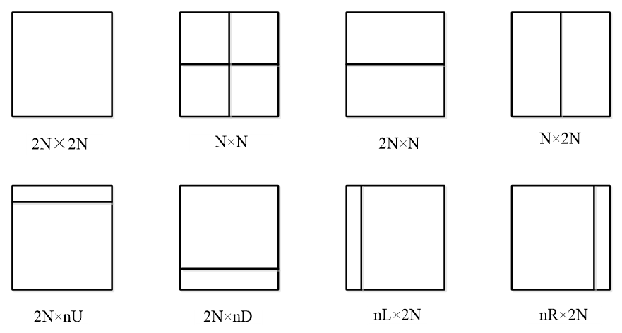
High efficiency video coding (HEVC) is approved by the Joint Collaborative Team on Video Coding which is composed of ITU Video Coding Experts Group and ISO/IEC Moving Picture Experts Group. HEVC can increase compression efficiency of 1080p video by about 50%. HEVC not only increases quality of video, but also saves a lot of bandwidth. We can enjoy higher quality 4K video, 3D Blu-ray, high-definition television program. Many new coding structures and coding technologies are adopted in HEVC compared with H.264, such as quadtree segmentation structure, 35 intra-prediction, advanced motion vector prediction, and so on. HEVC still adopts block-based hybrid coding framework. Inter-prediction makes use of temporal correlation to reduce temporal redundancy. First, we perform motion estimation to search for a block region which produces optimum correspondence to the current macroblock from reference frame. Then, the different information between matching block and current block is quantized and transformed, which leads to a entropy-coded and temporal-redundancy-reduced result. HEVC adopts coding tree unit (CTU) which is split into quadtree structure. CTU is divided into coding units (CUs). The CU size ranging from [TeX:] $$8 \times 8 \text { to } 64 \times 64.$$ The CU sizes of [TeX:] $$8 \times 8,16 \times 16,32 \times 32,64 \times 64$$ correspond to depth3, depth2, depth1, and depth0. Each CU is divided into prediction units (PUs). There are eight kinds of PUs for inter-prediction, including [TeX:] $$" \mathrm{~N} \times \mathrm{N}, \mathrm{N} \times 2 \mathrm{~N}, 2 \mathrm{~N} \times \mathrm{N}, 2 \mathrm{~N} \times 2 \mathrm{~N}, \mathrm{nR} \times 2 \mathrm{~N}, \mathrm{~nL} \times 2 \mathrm{~N}, 2 \mathrm{~N} \times \mathrm{nD} \text {, and } 2 \mathrm{~N} \times \mathrm{nU},"$$ ” Fig. 1 shows PU partition mode. To select the best CU size, CU is divided into eight PU types at each depth level [1,2]. All the CUs from [TeX:] $$8 \times 8 \text { to } 64 \times 64$$ and prediction modes are implemented to decide the best depth level. Inter-prediction takes up most of the time in the whole encoding process. We can improve encoding speed from both CU and PU to decrease the time spending during the course of inter prediction. Image processing technologies and statistical techniques are adopted to analyze the CU size range.
In [3], a fast inter-mode decision algorithm (FIMDA) analyzes the prediction mode distribution at each depth level, the motion vector and rate distortion cost of neighboring CUs select adaptively inter modes. The proposed efficient inter-prediction mode (EIPM) algorithms compute the priority of all inter-prediction modes. Motion estimation is executed in the high priority inter-prediction modes [4]. Lee et al. [5] propose fast CU size decision algorithms include early CU termination (ECUT), CU skip estimation (CUSE) and skip mode decision (SMD). In [6], a fast CU encoding algorithm is proposed. Spatio-temporal encoding parameters are used to decide CU partition. An algorithm by Huang et al. [7] adopts edge information of the partition to reduce computational complexity, and is especially suitable for simple texture and smooth movement. In [8], a fast reference frame selection algorithm makes use of content correlation between the sub-PU and parent PU to decrease computational burden. In [9], the algorithm utilizes statistical analysis to predict the rate distortion cost and bit cost, which skip unnecessary computation. Pareto-based method adopts fine- and medium-granularity encoding time to precisely set a limit to encoding time [10]. Efficient mode decision algorithm consists of asymmetric motion partition (AMP), symmetric motion partition (SMP), and square motion partition [11]. The proposed algorithm adopts CU classification technique to fast select CU size in [12]. The above methods take advantage of temporal-spatial correlation in the process of inter-mode decision. However, these methods also maintain computational complexity. Inter-prediction mode decision is the driving force of our research.
In the paper, the proposed algorithm includes fast CU depth range decision and fast PU partition mode decision. We can pre-estimate depth range to skip unnecessary CU depth level decision according to spatial-temporal correlation. We make use of depth difference between the co-located CU and the current CU to select PU partition mode range. The proposed algorithm can save about 50% of encoding time, while the video quality remains approximately the same.
In the following sections, the fast decision algorithm is introduced to analyze the inter-prediction mode. A fast CU depth range decision (FCDRD) is proposed in Section 2. In Section 3, temporal correlation of PU partition mode is verified. A fast PU partition mode decision (FPPMD) is proposed. In Section 4, the overall algorithm combines FCDRD with FPPMD. Section 5 describes simulation results.
2. Fast CU Depth Range Decision
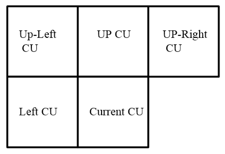
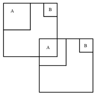
There are four cases of CU depth level, which are labelled by zero, one, two, and three. The probability that CU depth level of 0 or 1 is high for the smooth region, while the probability selection of 2 or 3 is high for complicated motion region [13]. We can pre-estimate depth range to skip unnecessary CU depth level decision. In [14], adaptive CU depth range makes use of depth level of the left and upper macroblocks to pre-estimate depth level range of the current macroblock. However, it does not save much time. The relationship of the current CU and its neighboring and co-located CU is heavy, as shown in Figs. 2 and 3. The paper proposes the algorithm which makes use of spatial and temporal correlation to predict depth range. [TeX:] $$D_{p r e}$$ is defined as follows:
(1)
[TeX:] $$D_{p r e}=\omega_{L} D_{L}+\omega_{U} D_{U}+\omega_{U-L} D_{U-L}++\omega_{U-R} D_{U-R}+\omega_{P} D_{P}$$where D represents the CU depth level, L, U, U-L, U-R, and P represent left, up, up-left, up-right, and the co-located position of the neighboring frame, respectively. To obtain more accurate prediction effect, rate distortion (RD) cost from spatial neighboring CUs and co-located CU is considered. An adaptive weight [TeX:] $$\omega$$ is proposed, as shown in formula (2). If the neighboring coding units of the current coding units is unavailable, [TeX:] $$D_{\text {pre }}$$ is set to 0 as starting value. We make use of [TeX:] $$D_{\text {pre }}$$ to select candidate depth level, as shown in Table 1.
(2)
[TeX:] $$\begin{gathered} \omega_{L}=\frac{R D_{L}}{R D_{L}+R D_{U}+R D_{U-L}+R D_{U-R}+R D_{P}} \\ \omega_{U}=\frac{R D_{U}}{R D_{L}+R D_{U}+R D_{U-L}+R D_{U-R}+R D_{P}} \\ \omega_{U-L}=\frac{R D_{U-L}}{R D_{L}+R D_{U}+R D_{U-L}+R D_{U-R}+R D_{P}} \\ \omega_{U \cdot R}=\frac{R D_{U-R}}{R D_{L}+R D_{U}+R D_{U-L}+R D_{U-R}+R D_{P}} \\ \omega_{P}=\frac{R D_{P}}{R D_{L}+R D_{U}+R D_{U-L}+R D_{U-R}+R D_{P}} \end{gathered}$$3. Fast PU Partition Mode Decision
The current CU and the co-located CU are alike. The current CU depth is in accordance with depth of the co-located CU, and then PU partition mode (PPM) range of the current CU may be determined by PPM of the co-located CU. Some unnecessary PPMs are skipped and computational complexity is reduced. For purpose of verifying temporal correlation, Traffic, BQTerrace, BQMall, and BQSquare are tested with QP=32. The first 2 seconds of each test sequences are adopted at the experiment.
The medial probability of PU with [TeX:] $$" 2 \mathrm{~N} \times 2 \mathrm{~N}, 2 \mathrm{~N} \times \mathrm{N}, \mathrm{N} \times 2 \mathrm{~N}, \mathrm{~N} \times \mathrm{N}, 2 \mathrm{~N} \times \mathrm{nU}, 2 \mathrm{~N} \times \mathrm{nD}, \mathrm{nL} \times 2 \mathrm{~N}, \mathrm{nR} \times 2 \mathrm{~N}^{\prime \prime}$$ is 97.90%, 0.66%, 0.84%, 0.06%, 0.14%, 0.11%, 0.16%, 0.13% from Table 2, when [TeX:] $$2 \mathrm{~N} \times 2 \mathrm{~N}$$ 2N is decided as the optimal PPM at the co-located CU. It is that the total probability selection of [TeX:] $$" 2 \mathrm{~N} \times 2 \mathrm{~N}, 2 \mathrm{~N} \times \mathrm{N}, \mathrm{N} \times 2 \mathrm{~N}^{\prime \prime}$$ is up to 99.4%. So when [TeX:] $$" 2 \mathrm{~N} \times 2 \mathrm{~N} "$$ is decided as the optimal PPM at the co-located CU, we only perform RD cost calculations on the three modes of [TeX:] $$" 2 \mathrm{~N} \times 2 \mathrm{~N}, 2 \mathrm{~N} \times \mathrm{N}^{\prime \prime} \text { " and " } \mathrm{N} \times 2 \mathrm{~N} . " \mathrm{RD}$$ cost of the current CU are calculated by the PPM of [TeX:] $$" 2 \mathrm{~N} \times 2 \mathrm{~N}, 2 \mathrm{~N} \times \mathrm{N}, \mathrm{N} \times 2 \mathrm{~N}, 2 \mathrm{~N} \times \mathrm{nU}, 2 \mathrm{~N} \times \mathrm{nD} \text { " }$$ and the rest PPMs are skipped when the PPM of co-located CU is [TeX:] $$\text { " } 2 \mathrm{~N} \times \mathrm{N} \text {." }$$ When the PPM of co-located CU is [TeX:] $$" \mathrm{~N} \times 2 \mathrm{~N}^{\prime \prime}$$ the candidate PPMs is [TeX:] $$" 2 \mathrm{~N} \times 2 \mathrm{~N}, 2 \mathrm{~N} \times \mathrm{N}, \mathrm{N} \times 2 \mathrm{~N}, \mathrm{~nL} \times 2 \mathrm{~N}, \mathrm{nR} \times 2 \mathrm{~N} \text { " }$$ at the current CU. The candidate PPMs of the current CU are [TeX:] $$" 2 \mathrm{~N} \times 2 \mathrm{~N}, 2 \mathrm{~N} \times \mathrm{N}, \mathrm{N} \times 2 \mathrm{~N}, \mathrm{~N} \times \mathrm{N}, "$$ when the PPM of co-located CU is [TeX:] $$" \mathrm{~N} \times \mathrm{N}_{.} \text {" }$$ When the PPM of co-located CU is [TeX:] $$\text { " } 2 \mathrm{~N} \times \mathrm{nD}"$$ the candidate PPMs are [TeX:] $$" 2 \mathrm{~N} \times 2 \mathrm{~N}, 2 \mathrm{~N} \times \mathrm{N}, \mathrm{N} \times 2 \mathrm{~N}, 2 \mathrm{~N} \times \mathrm{n} \mathrm{U}^{\prime \prime}$$ at the current CU. The candidate PPMs of the current CU are [TeX:] $$" 2 \mathrm{~N} \times 2 \mathrm{~N}, 2 \mathrm{~N} \times \mathrm{N}, \mathrm{N} \times 2 \mathrm{~N}, 2 \mathrm{~N} \times \mathrm{nD}, "$$ when the PPM of co-located CU is [TeX:] $$" 2 \mathrm{~N} \times \mathrm{nD} ."$$ When the PPM of co-located CU is [TeX:] $$" \mathrm{~nL} \times 2 \mathrm{~N}"$$ the candidate PPMs are [TeX:] $$" 2 \mathrm{~N} \times 2 \mathrm{~N}, 2 \mathrm{~N} \times \mathrm{N}, \mathrm{N} \times 2 \mathrm{~N}, \mathrm{~nL} \times 2 \mathrm{~N} "$$ ” at the current CU. The candidate PPMs of the current CU are [TeX:] $$" 2 \mathrm{~N} \times 2 \mathrm{~N}, 2 \mathrm{~N} \times \mathrm{N}, \mathrm{N} \times 2 \mathrm{~N}, \mathrm{nR} \times 2 \mathrm{~N} "$$ when the PPM of co-located CU is [TeX:] $$" \mathrm{nR} \times 2 \mathrm{~N} "$$ We make use of temporal correlation to decrease the number of the PPMs and complexity of PPM decision.
Table 2.
| Best PU mode of the co-located CU | PPM of the current CU (%) | |||||||
|---|---|---|---|---|---|---|---|---|
| [TeX:] $$2 N \times 2 N$$ | [TeX:] $$2 N \times N$$ | [TeX:] $$\mathbf{N} \times \mathbf{2 N}$$ | [TeX:] $$\mathbf{N} \times \mathbf{N}$$ | [TeX:] $$2 \mathbf{N} \times \mathbf{n U}$$ | [TeX:] $$2 \mathrm{~N} \times \mathrm{nD}$$ | [TeX:] $$n L \times 2 N$$ | [TeX:] $$\mathrm{nR} \times 2 \mathrm{~N}$$ | |
| [TeX:] $$2 N \times 2 N$$ | 97.90 | 0.66 | 0.84 | 0.06 | 0.14 | 0.11 | 0.16 | 0.13 |
| [TeX:] $$2 \mathrm{~N} \times \mathrm{N}$$ | 93.68 | 2.40 | 2.22 | 0.25 | 0.35 | 0.50 | 0.34 | 0.26 |
| [TeX:] $$\mathrm{N} \times 2 \mathrm{~N}$$ | 94.39 | 1.83 | 2.94 | 0.34 | 0.31 | 0.19 | 0.42 | 0.48 |
| [TeX:] $$\mathrm{N} \times \mathrm{N}$$ | 95.78 | 0.97 | 2.13 | 0.26 | 0.24 | 0.20 | 0.18 | 0.24 |
| [TeX:] $$2 \mathrm{~N} \times \mathrm{nU}$$ | 93.39 | 2.25 | 2.14 | 0.31 | 0.85 | 0.37 | 0.35 | 0.34 |
| [TeX:] $$2 N \times n D$$ | 94.23 | 2.26 | 1.90 | 0.16 | 0.26 | 0.62 | 0.34 | 0.23 |
| [TeX:] $$\mathrm{n} L \times 2 \mathrm{~N}$$ | 92.67 | 1.63 | 3.42 | 0.28 | 0.23 | 0.24 | 0.96 | 0.57 |
| [TeX:] $$\mathrm{nR} \times 2 \mathrm{~N}$$ | 92.97 | 1.52 | 3.40 | 0.22 | 0.34 | 0.28 | 0.48 | 0.79 |
4. The Overall Algorithm
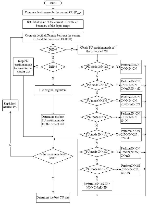
Firstly, depth range of the current CU is calculated by formula (1). Secondly, we calculate depth difference between the co-located CU and the current CU. If the depth difference is 0, PPM range is selected at the current CU by the PPM of the co-located CU. If the depth difference is 1 or 2, PPM decision is performed by HM original algorithm. If the depth level difference is 3, PPM traversed by the current CU are skipped. Fig. 4 shows flow diagram of the whole algorithm.
5. Experimental Results
In order to verify the property of the whole algorithm, FCDRD and FPPMD are performed on HM14.0 reference software. HEVC standardization has been performed for two different scenarios, random access (RA) and low delay (LD). Entertainment applications are supported by random access. Interactive applications are restrained by low delay. Table 3 shows the test sequences are used under both RA and LD conditions. Each test sequence is performed with QP=37, 32, 27, and 22. The experimental results are measured in terms of Bjontegaard delta peak signal-to-noise ratio (BDPSNR), Bjontegaard delta bitrate (BDBR), and time saving (TS). TS represents the saved coding time compared to HM14.0. A positive or negative value of TS indicates the increase or decrease of time.
Table 3.
| Sequence | Resolution | Frame rate (fps) |
|---|---|---|
| Traffic | [TeX:] $$2560 \times 1600(\mathrm{~A})$$ | 30 |
| PeopleOnStreet | [TeX:] $$2560 \times 1600(\mathrm{~A})$$ | 30 |
| Kimonol | [TeX:] $$1920 \times 1080(B)$$ | 24 |
| ParkScene | [TeX:] $$1920 \times 1080(B)$$ | 24 |
| Cactus | [TeX:] $$1920 \times 1080(B)$$ | 50 |
| BQTerrace | [TeX:] $$1920 \times 1080(\mathrm{~B})$$ | 60 |
| BasketballDrill | [TeX:] $$832 \times 480(\mathrm{C})$$ | 50 |
| BQMall | [TeX:] $$832 \times 480(\mathrm{C})$$ | 60 |
| PartyScene | [TeX:] $$832 \times 480(\mathrm{C})$$ | 50 |
| BasketballPass | [TeX:] $$416 \times 240 \text { (D) }$$ | 50 |
| BlowingBubbles | [TeX:] $$416 \times 240 \text { (D) }$$ | 50 |
| BQSquare | [TeX:] $$416 \times 240 \text { (D) }$$ | 60 |
| SlideShow | [TeX:] $$1280 \times 720(\mathrm{~F})$$ | 30 |
| SlideEditing | [TeX:] $$1280 \times 720(\mathrm{~F})$$ | 20 |
| ChinaSpeed | [TeX:] $$1024 \times 768(\mathrm{~F})$$ | 30 |
| BasketballDrillText | [TeX:] $$832 \times 480(\mathrm{~F})$$ | 50 |
The experiment result is shown in Tables 4 and 5. The FCDRD algorithm can save coding time by 31.3%–34.6% on average, while BDPSNR slightly lose 0.07–0.11 dB and BDBR slightly increase 1.00%–1.34% under both RA and LD conditions. The procedures of CU depth decision skip some unnecessary depth levels for test sequences. The SlideEditing sequence saves time by a maximum of 42.7%. The BlowingBubbles sequence saves time by a minimum of 19.8%. The FPPMD algorithm reduces the number of PU candidate modes traversed. Since the low-activity sequences have simple motion characteristics, the number of candidate modes traversed by the low activity sequences is less than that of the high activity sequences. The FPPMD can decrease the coding time of SlideEditing sequence by up to 36.4% (RA) and PeopleOnStreet (RA) sequence by a minimum of 10.2%. The average BDPSNR is decreased by 0.02–0.05 dB and the average BDBR is increased by 0.66%–0.74% under both RA and LD conditions, which are negligible. The proposed overall algorithm which combines the FCDRD algorithm with the FPPMD algorithm is applied to all test sequences. The proposed overall algorithm can save 41.9% and 44.3% coding time compared with HM14.0, while 0.10–0.16 dB PSNR loss and 1.49%–1.88% bitrate increment can be ignored. Tables 4 and 5 show results of FCDRD, FPPMD, and overall algorithm compared with HM14.0.
Table 4.
| Test sequence | FCDRD | FPPMD | The overall algorithm | ||||||
|---|---|---|---|---|---|---|---|---|---|
| BDPSNR (dB) | BDBR (%) | TS (%) | BDPSNR (dB) | BDBR (%) | TS (%) | BDPSNR (dB) | BDBR (%) | TS (%) | |
| Traffic | -0.07 | 1.10 | -38.1 | -0.06 | 0.84 | -31.1 | -0.13 | 1.78 | -54.2 |
| PeopleOnStreet | -0.05 | 0.70 | -25.4 | -0.04 | 0.95 | -10.2 | -0.09 | 1.64 | -27.7 |
| Kimonol | -0.09 | 0.56 | -32.7 | -0.02 | 0.78 | -23.8 | -0.08 | 1.32 | -40.7 |
| ParkScene | -0.05 | 1.21 | -38.3 | -0.04 | 0.67 | -29.2 | -0.09 | 1.65 | -50.3 |
| Cactus | -0.07 | 0.80 | -39.5 | -0.03 | 0.59 | -26.1 | -0.10 | 1.23 | -47.1 |
| BQTerrace | -0.04 | 0.76 | -42.4 | -0.04 | 0.34 | -28.4 | -0.08 | 0.96 | -53.2 |
| BasketballDrill | -0.07 | 2.01 | -31.7 | -0.04 | 0.53 | -24.2 | -0.11 | 2.15 | -41.4 |
| BQMall | -0.01 | 0.85 | -31.1 | -0.05 | 0.78 | -35.5 | -0.06 | 1.48 | -44.8 |
| PartyScene | -0.06 | 0.87 | -35.6 | -0.03 | 0.86 | -26.7 | -0.09 | 1.56 | -45.6 |
| BasketballPass | -0.12 | 1.98 | -33.7 | -0.05 | 0.45 | -20.5 | -0.17 | 2.23 | -38.9 |
| BlowingBubbles | -0.07 | 0.85 | -23.4 | -0.04 | 0.37 | -18.9 | -0.11 | 1.06 | -32.8 |
| BQSquare | -0.12 | 2.64 | -29.6 | -0.08 | 1.02 | -29.0 | -0.20 | 3.34 | -35.6 |
| SlideShow | -0.11 | 1.98 | -41.2 | -0.07 | 0.80 | -32.3 | -0.18 | 2.45 | -55.1 |
| SlideEditing | -0.16 | 2.01 | -45.4 | -0.10 | 1.03 | -36.4 | -0.26 | 2.87 | -59.7 |
| ChinaSpeed | -0.29 | 1.36 | -32.6 | -0.08 | 0.83 | -20.2 | -0.37 | 2.01 | -40.4 |
| BasketballDrillText | -0.33 | 1.75 | -32.2 | -0.06 | 0.98 | -32.5 | -0.39 | 2.34 | -41.3 |
| Average | -0.11 | 1.34 | -34.6 | -0.05 | 0.74 | -26.6 | -0.16 | 1.88 | -44.3 |
Table 5.
| Test sequence | FCDRD | FPPMD | The overall algorithm | ||||||
|---|---|---|---|---|---|---|---|---|---|
| BDPSNR (dB) | BDBR (%) | TS (%) | BDPSNR (dB) | BDBR (%) | TS (%) | BDPSNR (dB) | BDBR (%) | TS (%) | |
| Traffic | - | - | - | - | - | - | - | - | - |
| PeopleOnStreet | - | - | - | - | - | - | - | - | - |
| Kimonol | -0.05 | 0.24 | -28.3 | -0.00 | 0.70 | -22.9 | -0.06 | 0.90 | -38.7 |
| ParkScene | -0.01 | 0.98 | -33.5 | -0.01 | 0.62 | -28.4 | -0.02 | 1.45 | -45.6 |
| Cactus | -0.03 | 0.54 | -35.2 | -0.00 | 0.53 | -23.3 | -0.03 | 1.03 | -39.4 |
| BQTerrace | -0.02 | 0.34 | -38.7 | -0.01 | 0.21 | -27.5 | -0.03 | 0.46 | -49.4 |
| BasketballDrill | -0.03 | 1.61 | -26.6 | -0.02 | 0.64 | -23.1 | -0.04 | 1.95 | -42.7 |
| BQMall | -0.01 | 0.67 | -28.5 | -0.02 | 0.76 | -31.9 | -0.03 | 1.28 | -43.7 |
| PartyScene | -0.03 | 0.45 | -29.7 | -0.00 | 0.73 | -24.2 | -0.02 | 1.06 | -41.5 |
| BasketballPass | -0.07 | 1.08 | -31.2 | -0.02 | 0.34 | -19.6 | -0.09 | 1.23 | -36.2 |
| BlowingBubbles | -0.02 | 0.65 | -19.8 | -0.02 | 0.36 | -16.9 | -0.03 | 0.86 | -30.6 |
| BQSquare | -0.04 | 1.97 | -22.4 | -0.04 | 0.91 | -26.3 | -0.06 | 2.54 | -34.4 |
| SlideShow | -0.05 | 1.76 | -39.5 | -0.05 | 0.50 | -29.2 | -0.09 | 2.14 | -49.3 |
| SlideEditing | -0.18 | 1.47 | -42.7 | -0.08 | 1.00 | -33.7 | -0.26 | 2.36 | -54.8 |
| ChinaSpeed | -0.24 | 0.96 | -31.1 | -0.03 | 0.90 | -18.4 | -0.34 | 1.67 | -39.5 |
| BasketballDrillText | -0.23 | 1.29 | -30.4 | -0.02 | 0.99 | -28.1 | -0.24 | 1.94 | -40.2 |
| Average | -0.07 | 1.00 | -31.3 | -0.02 | 0.66 | -25.2 | -0.10 | 1.49 | -41.9 |
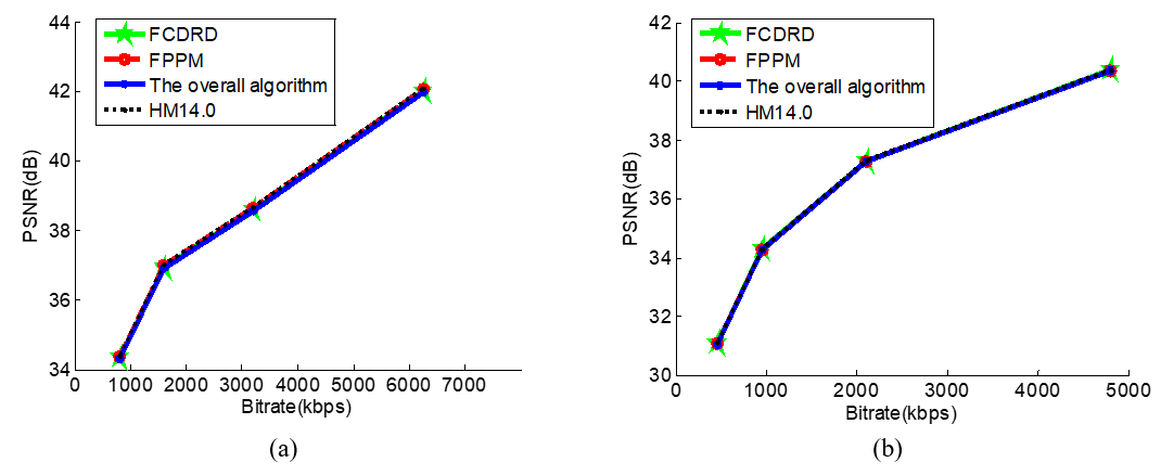
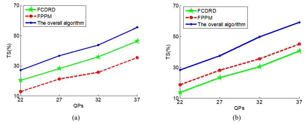
Figs. 5 and 6 show the coding performance of Kimonol and BQMall using different QPs under both RA and LD conditions. The RD curves between the proposed algorithms and the HM14.0 are approximated. However, the proposed algorithms can save plenty time.
6. Conclusion
To reduce computational complexity, the proposed whole algorithm which consists of FCDRD and FPPMD is performed on HM14.0. FCDRD making use of depth level of spatially and temporally adjacent CU to predict depth level range of the current CU. FPPMD skips unnecessary mode selection according to the depth relationship of the corresponding position CU and the current CU. The proposed whole algorithm reduces 41.9%–44.3% of encoding time on average, while RD performance is approximately unchanged. In this paper, we only use the spatial-temporal correlation to obtain prediction mode of CU and PU. In the future work, other motion parameters are considered, so that CU and PU can be predicted more accurately.
Acknowledgement
This work is supported by the Emerging Engineering Project of Anhui Polytechnic University (No. 2018xgksfkc08), the National Natural Science Foundation of China (No. 61572033), Key Projects of Natural Science Research Fund of Anhui Province (No. KJ2015A311), the Open Research Fund of Anhui Key Laboratory of Detection Technology and Energy Saving Devices, Anhui Polytechnic University (No. DTESD2020B07), and Anhui Polytechnic University research fund (No. Xjky2020121, Xjky2020 029).
References
- 1 G. J. Sullivan, J. R. Ohm, "Recent developments in standardization of high efficiency video coding (HEVC)," in Proceedings of SPIE 7798: Applications of Digital Image Processing XXXIII. Bellingham, W A: International Society for Optics and Photonics, 2010;doi:[[[10.1117/12.863486]]]
- 2 G. J. Sullivan, T. Wiegand, "Video compression-from concepts to the H. 264/A VC standard," in Proceedings of the IEEE, 2005;vol. 93, no. 1, pp. 18-31. custom:[[[-]]]
- 3 L. Shen, Z. Zhang, Z. Liu, "Adaptive inter-mode decision for HEVC jointly utilizing inter-level and spatiotemporal correlations," IEEE Transactions on Circuits and Systems for Video Technology, vol. 24, no. 10, pp. 1709-1722, 2014.doi:[[[10.1109/TCSVT.2014.2313892]]]
- 4 A. Lee, D. Jun, J. Kim, J. S. Choi, J. Kim, "Efficient inter prediction mode decision method for fast motion estimation in high efficiency video coding," ETRI Journal, vol. 36, no. 4, pp. 528-536, 2014.doi:[[[10.4218/etrij.14.0113.0087]]]
- 5 J. Lee, S. Kim, K. Lim, S. Lee, "A fast CU size decision algorithm for HEVC," IEEE Transactions on Circuits and Systems for Video Technology, vol. 25, no. 3, pp. 411-421, 2014.doi:[[[10.1109/TCSVT.2014.2339612]]]
- 6 S. Ahn, B. Lee, M. Kim, "A novel fast CU encoding scheme based on spatiotemporal encoding parameters for HEVC inter coding," IEEE Transactions on Circuits and Systems for Video Technology, vol. 25, no. 3, pp. 422-435, 2015.doi:[[[10.1109/TCSVT.2014.2360031]]]
- 7 X. Huang, Q. Zhang, X. Zhao, W. Zhang, Y. Zhang, Y. Gan, "Fast inter-prediction mode decision algorithm for HEVC," SignalImage and Video Processing, vol. 11, pp. 33-40, 2017.doi:[[[10.1007/s11760-016-0887-4]]]
- 8 Z. Pan, P. Jin, J. Lei, Y. Zhang, X. Sun, S. Kwong, "Fast reference frame selection based on content similarity for low complexity HEVC encoder," Journal of Visual Communication and Image Representation, vol. 40, pp. 516-524, 2016.doi:[[[10.1016/j.jvcir.2016.07.018]]]
- 9 S. H. Jung, H. W. Park, "A fast mode decision method in HEVC using adaptive ordering of modes," IEEE Transactions on Circuits and Systems for Video Technology, vol. 26, no. 10, pp. 1846-1858, 2016.doi:[[[10.1109/TCSVT.2015.2473303]]]
- 10 G. Correa, P. A. Assuncao, L. V. Agostini, L. A. da Silva Cruz, "Pareto-based method for high efficiency video coding with limited encoding time," IEEE Transactions on Circuits and Systems for Video Technology, vol. 26, no. 9, pp. 1734-1745, 2016.doi:[[[10.1109/TCSVT.2015.2469533]]]
- 11 J. V anne, M. Viitanen, T. D. Hamalainen, "Efficient mode decision schemes for HEVC inter prediction," IEEE Transactions on Circuits and Systems for Video Technology, vol. 24, no. 9, pp. 1579-1593, 2014.doi:[[[10.1109/TCSVT.2014.2308453]]]
- 12 T. Mallikarachchi, A. Fernando, H. K. Arachchi, "Fast coding unit size selection for HEVC inter prediction," in Proceedings of 2015 IEEE International Conference on Consumer Electronics (ICCE), Las V egas, NV, 2015;pp. 457-458. doi:[[[10.1109/icce.2015.7066485]]]
- 13 L. Shen, Z. Liu, X. Zhang, W. Zhao, Z. Zhang, "An effective CU size decision method for HEVC encoders," IEEE Transactions on Multimedia, vol. 15, no. 2, pp. 465-470, 2013.doi:[[[10.1109/TMM.2012.2231060]]]
- 14 X. Li, J. An, X. Guo, and S. Lei, in the Meeting report of the Joint Collaborative Team on Video Coding (JCT-VC) of ITU-T WP3/16 and ISO/IEC JTC 1/SC 29/WG 11, Geneva, Switzerland, 2011 (Online). Available:, https://www.itu.int/wftp3/av-arch/jctvc-site/2011_03_E_Geneva/JCTVC-E_Notes_d8.doc
