Seungmin Lee and Daejin Park*
Improved Dynamic Programming in Local Linear Approximation Based on a Template in a Lightweight ECG Signal-Processing Edge Device
Abstract: Interest is increasing in electrocardiogram (ECG) signal analysis for embedded devices, creating the need to develop an algorithm suitable for a low-power, low-memory embedded device. Linear approximation of the ECG signal facilitates the detection of fiducial points by expressing the signal as a small number of vertices. However, dynamic programming, a global optimization method used for linear approximation, has the disadvantage of high complexity using memoization. In this paper, the calculation area and memory usage are improved using a linear approximated template. The proposed algorithm reduces the calculation area required for dynamic programming through local optimization around the vertices of the template. In addition, it minimizes the storage space required by expressing the time information using the error from the vertices of the template, which is more compact than the time difference between vertices. When the length of the signal is L, the number of vertices is N, and the margin tolerance is M, the spatial complexity improves from O(NL) to O(NM). In our experiment, the linear approximation processing time was 12.45 times faster, from 18.18 ms to 1.46 ms on average, for each beat. The quality distribution of the percentage root mean square difference confirms that the proposed algorithm is a stable approximation.
Keywords: Device Discovery , Partition-Based , RDM
1. Introduction
With recent software and hardware technology developments, healthcare monitoring technologies have been implemented using bio-signals measured by embedded devices [1,2]. Healthcare research is being actively conducted in various fields such as sensor data acquisition, sensor data-transmission technology, and sensor data analysis [3,4]. Based on this research, applied technologies are being used in various fields such as human activity, care for older adults, security, and smart homes [5]. In particular, as interest in health increases due to prolonged average life spans, healthcare systems as daily wearable devices have been in the spotlight [6,7]. In addition, the mortality rate of heart disease is increasing due to the prolonged average lifespans, so research is increasing on bio-signal monitoring and analysis systems for diagnosing early heart disease.
Among bio-signals, studying electrocardiogram (ECG) signal analysis is useful for the early prevention of heart disease. Because an ECG signal measures electrical signals generated according to the heart activity, it is the most useful biological signal for analyzing arrhythmia, which requires abnormal beat detection and analysis. However, because abnormal beats are rare, long-term measurement lasting longer than 24 hours is required to detect them. In addition, a high sampling frequency of 250 Hz or 360 Hz is generally used to obtain accurate feature values to detect and analyze abnormal beats. Therefore, storing and transmitting the original signal incurs high costs, requiring an effective signal-compression method [8,9].
Furthermore, to increase the operating time of wireless measuring equipment, research on signal compression is needed to reduce power consumption by minimizing communication time. Fig. 1 shows an example of a Holter monitor, which is a representative wired measuring equipment, and a wireless measuring device using the Bluetooth function of a smartphone.
As shown in Fig. 1, wireless measuring equipment reduces the inconvenience of Holter monitors. Therefore, a signal-compression technique is required to store and transmit the signals used in real-time operation in embedded equipment.
In existing studies, the linear approximation method using dynamic programming is an algorithm that expresses the ECG signal as a straight line connecting a small number of vertices and emphasizes the feature values of the fiducial point to facilitate its detection [10,11]. This algorithm can be used as a signal-compression method because it expresses a signal with a small number of vertices. In particular, the processing time and memory usage of dynamic programming to optimize the approximation error are optimized based on the characteristics of the ECG signal, making real-time operation possible even in embedded devices [12,13]. The improved linear approximation has a spatial complexity of O(LN), where the length of the signal is L and the number of vertices is N. However, the approximation proceeds independently according to the beat, and the characteristic of the ECG signal in which a similar beat is repeated is not used effectively. Thus, the method is less efficient than compression methods in the frequency domain, such as wavelet transform [14].
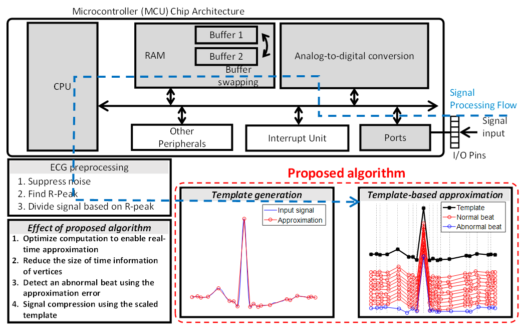
In this paper, we propose a local linear approximation method within the margin (M) range around the template vertices. The proposed method proceeds based on the similarity of the vertices because the normal beat, which occupies most of the ECG signal, is repeated in a similar shape. That is, the amount of data is minimized by recording the time difference from the template vertex. Because the range of the location information of the vertices is limited by the margin, the cost and base matrices for memoization in dynamic programming are reduced, reducing the spatial complexity from O(LN) to O(MN). Accordingly, the amount of computation decreases proportionally. Although the margin limits the vertex range, the approximation error increases, but the quality of the percentage root-mean-square difference (PRD) stabilizes. Fig. 2 summarizes the algorithm flow and effects of the proposed method.
This paper is composed as follows. Section 2 introduces the composition and characteristics of the ECG signal, and Section 3 explains the existing linear approximation method. After explaining the proposed algorithm in Section 4, we confirm its performance through experiments in Section 5, and we conclude this paper in Section 6.
2. Composition and Characteristics of the ECG Signal
2.1 Composition of the ECG Signal
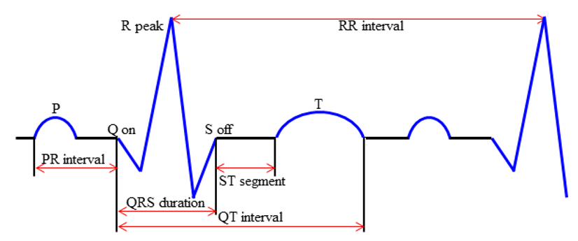
The atrium and ventricle contract during depolarization and relax during repolarization. At this time, an ECG signal is obtained by measuring the electrical signal, and the P wave, QRS complex, and T wave are periodically repeated. Arrhythmia affects the beat, causing abnormal beats, which include changes in the period or deformations of the shape. Therefore, ECG signal analysis is used to detect and analyze abnormal beats. The feature values are obtained from the time interval or amplitude difference between the fiducial points of each waveform, generally referring to the start point (onset), the endpoint (offset), and the peak of each waveform. Fig. 3 shows the fiducial points and feature values of the ECG signals commonly used in ECG signal analysis.
2.2 Abnormal Beat in an ECG Signal
ANSI-AAMI EC57:1998 by the American Medical Association classifies arrhythmia into five categories: a normal beat (N), upper ventricular arrhythmia beat (S), ventricular arrhythmia beat (V), mixed arrhythmia beat (F), and unclassified beat (Q). PhysioNet provides a variety of arrhythmia databases and categorizes the beats into 19 categories. Table 1 shows the distribution of 48 recordings measured for 30 minutes each in the MIT-BIH Arrhythmia Database (MIT-BIH ADB), provided by PhysioNet, classified into 19 categories [15].
The left and right bundle branch block (L, R) and the pacemaker beat (/) replace the normal beat. That is, approximately 89% of the beat is generated as a normal beat. In some of the data, even though the data are 30 minutes long, the rate of normal beats is 99% or 100%. As such, most of the ECG signals comprise a normal beat that repeats a similar shape.
Table 1.
| Code | Total number | Description | Class |
|---|---|---|---|
| N | 75,052 | Normal beat | Normal |
| L | 8,075 | Left bundle branch block beat | Bundle branch block |
| R | 7,259 | Right bundle branch block beat | |
| B | 0 | Bundle branch block beat | |
| A | 2,546 | Atrial premature beat | Premature |
| a | 150 | Aberrated atrial premature beat | |
| J | 83 | Junctional premature beat | |
| S | 2 | Supraventricular premature beat | |
| V | 7,130 | Premature ventricular contraction | |
| r | 0 | R-on-T premature ventricular contraction | |
| F | 803 | Fusion of ventricular and normal beat | |
| e | 16 | Atrial escape beat | Escape |
| j | 229 | Junctional escape beat | |
| n | 0 | Supraventricular escape beat | |
| E | 106 | Ventricular escape beat | |
| / | 7,028 | Paced beat | Paced |
| f | 982 | Fusion of paced and normal beat | |
| Q | 33 | Unclassifiable beat | Else |
| ? | 0 | Beat not classified during learning |
2.3 Preprocessing of the ECG Signal
When measuring the ECG signals for an extended time, noise is also picked up from various external stimuli. Accordingly, preprocessing is required to suppress the noise. In addition, it is necessary to separate the beat first to distinguish between a normal beat and an abnormal beat. R-peak detection is a good approach for this separation.
2.3.1 Noise reduction
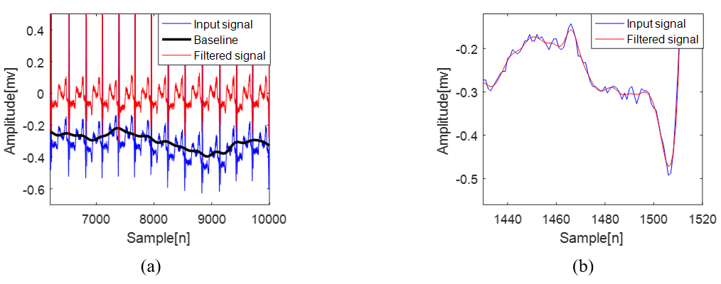
Noise generated during the ECG signal-measurement process can have various causes. First, power noise and breathing can cause regularly generated high- and low-frequency noises. Irregular noises include activity from surrounding muscles and noise from external electronic equipment [16–19]. In this paper, a third-order Butterworth band-pass filter of 1–25 Hz was applied to suppress high-frequency noise over 25 Hz caused by power noise and low-frequency noise near 0.1 Hz resulting from breathing.
Fig. 4 shows a raw signal, including noise, and the filtered signal.
2.3.2 R-peak detection
The R-peak represents the peak of the QRS complex and is generally the fiducial point with the highest amplitude in the beat. Its detection is easier and more accurate than detection of other fiducial points, so it is used as a standard to classify the beat [20]. Pan’s method [21] is a representative QRS complex detection, in which auxiliary signals are obtained using a differential signal, a square signal, and an average filter, based on the QRS complex having a large amplitude change. The QRS complex is detected using an adaptive threshold based on these auxiliary signals. Then, the R-peak is detected based on the highest amplitude value. Fig. 5 shows the auxiliary signal and threshold generated by Pan’s method, as well as the R-peak detected using the highest amplitude value within the QRS complex.
Fig. 5.
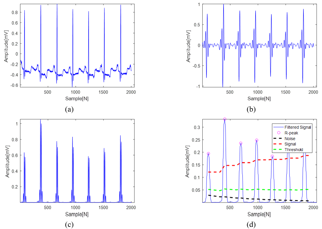
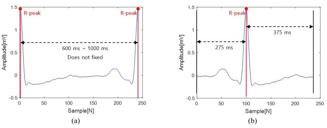
Pan’s method [21] can be used in real-time processing and is widely used in various ECG signal-processing methods due to its high detection rate of the QRS complex. Pan’s method can detect the R-peak and separate the beat. Fig. 6 shows the two methods of beat separation.
The beat is divided into data within the RR interval from one R-peak to the next R-peak, with the existing linear approximation method based on this region. However, because the RR interval does not have a constant beat, it is difficult to determine the template’s length. The linear interpolation algorithm was proposed to solve this problem by adjusting the signal lengths and making them the same. This is suitable for determining a representative beat signal but not for detecting abnormal beats, which requires individual analysis of each signal or information to be transmitted through signal compression due to the large amount of erroneous detection caused by signal distortion.
Another method is to divide the beat to include all the major waveform information within each beat by acquiring information from 275 ms before to 375 ms after the R-peak [22]. In this paper, because we use a template with linear approximation, we used beat separation centering on the R-peak.
3. Linear Approximation of the ECG Signal
3.1 Linear Approximation Step
Linear approximation of the ECG signal consists of three steps: curvature-based linear approximation, sequential linear approximation, and error optimization.
3.1.1 Curvature-based linear approximation
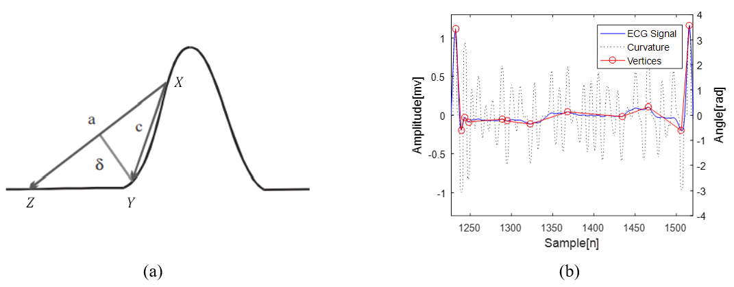
First, a point with a large curvature is obtained as the initial vertex using curvature-based linear approximation [23]. The curvature is the amount by which a curve deviates from a straight line. In this paper, it is calculated as in Eq. (1), using the included angle between three points:
(1)
[TeX:] $$\delta(Y ; X, Z)=\frac{\vec{a} \times \vec{c}}{|\vec{a}|}=\frac{\left(x_{1}-z_{1}\right)\left(x_{2}-y_{2}\right)-\left(x_{2}-z_{2}\right)\left(x_{1}-y_{1}\right)}{\sqrt{\left(x_{1}-z_{1}\right)+\left(x_{2}-z_{2}\right)^{2}}}, \quad x_{1}>y_{1}>z_{1}$$Fig. 7 shows the concept of the curvature calculation process and an example of an approximated input signal.
Fig. 7.
3.1.2 Sequential linear approximation
Curvature-based linear approximation effectively expresses a fiducial point as the initial vertex because the point has a large curvature. However, if the amplitude change of the waveform is minimal, it may not be acquired as the initial vertex, as shown in QRS-onset and P-offset in Fig. 7. To correct this, additional vertices are obtained for the inside of each initial vertex using sequential linear approximation [24]. Fig. 8 shows the concept of the sequential linear approximation process and an example of an approximated signal of Fig. 7(b).
Fig. 8.
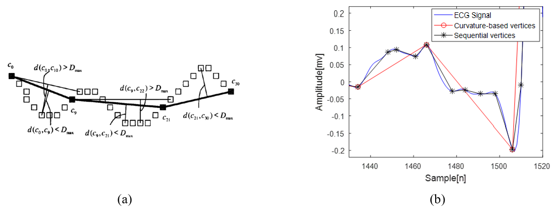
As shown in Fig. 8(a), a vertex is added when the error exceeds the threshold [TeX:] $$D_{\max },$$ and the signal was effectively approximated, as shown in Fig. 8(b).
3.1.3 Error optimization
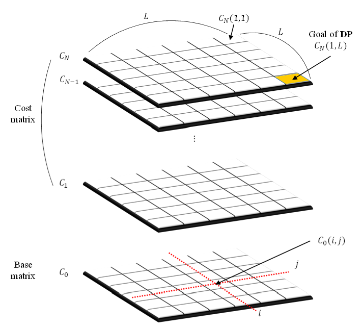
Global error optimization calculates the costs for all cases and detects the minimum case as the optimization result. Therefore, the problem of optimizing the position of N vertices for L samples generally has a complexity of [TeX:] $$O\left(L^{N}\right).$$ Dynamic programming [10] is a global optimization technique in which the optimal path between two points is optimized based on the Bellman principle as the globally optimal path between any two points on the globally optimal path. The recursive approach simplifies and optimizes the problem, especially using memoization to remember the computational results, eliminating redundant operations. Dynamic programming enables high-speed global optimization, but it requires additional memory for memoization, consisting of cost and base matrices. In this case, the size of the cost and base matrices required for memoization is [TeX:] $$O\left(L^{2} N\right).$$ Fig. 9 shows the cost and base matrices used for the memoization of dynamic programming.
For a signal with length L, the optimization of the partial signal from i to j, including the k vertices, is recursively calculated as in Eq. (2):
(2)
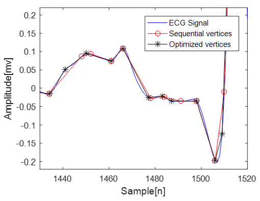
[TeX:] $$C_{k}(i, j)=\min _{v_{k} \in[1, \cdots, L]}\left(C_{k-1}\left(i, v_{k}\right)+C_{0}\left(v_{k}, j\right)\right)$$where [TeX:] $$v_{k}$$ denotes the position of the kth vertex, and when k is [TeX:] $$0, C_{0}(i, j)$$ is calculated as an error between the input signal and the line connecting the ith sample and jth sample. Fig. 10 shows the results of optimization using dynamic programming of Fig. 8(b).
As shown in Fig. 10, the signal is well represented with a small number of vertices, and dynamic programming reduces the error.
3.2 Optimization of Dynamic Programming
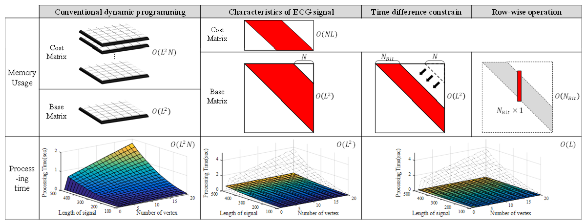
Dynamic programming is a global optimization method proposed by Bellman that optimizes the problem through a top-down recursive approach. Using memoization to store the operation’s results in the recursion process removes redundant operations, and global optimization occurs relatively quickly. However, the size of the cost and base matrices required for memoization has a time and spatial complexity of [TeX:] $$O\left(L^{2} N\right)$$ depending on the length of the signal L and the number of vertices N, making real-time processing difficult. To improve this, Lee [12] optimizes the calculation of the cost and base matrices based on the ECG signal’s characteristics, thereby improving the performance and enabling real-time operation, even in an embedded device. Fig. 11 shows the results of improving the spatial complexity of the cost and base matrices used in dynamic programming.
The following is a description of each step in Fig. 11.
1) Improvement based on characteristics of ECG signals
First, because the approximation error of the ECG signal is not affected by the measurement direction, the cost and base matrices are symmetric. In addition, because each vertex of the ECG signal is selected according to the passage of time, the vertices’ time information increases monotonically. The first and last vertices are fixed as the initial vertices corresponding to both ends of the input signal. Therefore, in [TeX:] $$C_{k}(i, j)$$ of Eq. (2), i is always 1, and the existing cost matrix [TeX:] $$C_{k}(i, j)$$ is expressed as [TeX:] $$C(k, j)$$ in Eq. (3):
(3)
[TeX:] $$C(k, j)=\min _{1<v_{k}<j}\left(C\left(k-1, v_{k}\right)+C_{0}\left(v_{k}, j\right)\right)$$By expressing [TeX:] $$C_{k}(1, j) \text { as } C(k, j),$$ the cost matrix of size [TeX:] $$O\left(L^{2} N\right)$$ ) is reduced to size O(NL). Thus, C(N,L) is an optimized error value when N additional vertices exist between the first sample and the Lth (last) sample, and it represents the result of dynamic programming. In addition, the existing dynamic programming method optimizes by performing calculations in a recursive, top-down method. However, improving the cost matrix fixes the area required for calculation. Therefore, it can be optimized through a bottom-up operation without a recursive approach.
2) Add a limit of the time difference between vertices
Because the ECG signal is measured for an extended time, many data bits are required to record the vertices’ time information. To improve this, the amount of information is minimized by representing the vertex information as the time difference from the previous vertex. The maximum interval between the vertices is limited by the number of bits indicating the time difference between the vertices. Accordingly, the operation area of the base matrix for recording the approximation error between two adjacent vertices is reduced to the limit based on the number of bits. The cost matrix C(k,j) is calculated only when the interval between the kth vertex and the (k+1)th vertex does not exceed N_Bit, as in Eq. (4):
(4)
[TeX:] $$C(k, j)=\min _{v_{k+1}-N_{B i t} \leq v_{k}<v_{k+1}}\left(C\left(k-1, v_{k}\right)+C_{0}\left(v_{k}, j\right)\right)$$The computation of the base matrix is reduced, as shown in Fig. 11, because the time difference between the two vertices is limited by [TeX:] $$N_{B i t}.$$
3) Row-wise operation
The first row of the cost matrix is calculated based on the result of the base matrix operation. Similarly, the (k+1)th row of the cost matrix is sequentially calculated using the kth row of the cost matrix and base matrix’s corresponding components, which is repeated until the Nth row. This row-wise operation requires a call to a base matrix with a large area, making it difficult to improve the base matrix. However, when each component of the cost matrix is calculated in a column-wise operation, the called base matrix is sequentially called column by column. That is, the jth column of the base matrix is only used to calculate the cost matrix’s jth column. Thus, the base matrix [TeX:] $$C_{0}\left(v_{k}, j\right)$$ in Eq. (4) can be expressed as Eq. (5):
(5)
[TeX:] $$C(k, j)=\min _{v_{k+1}-N_{B i t} \leq v_{k}<v_{k+1}}\left(C\left(k-1, v_{k}\right)+C_{0}^{j}\left(v_{k}-\left(v_{k+1}-N_{B i t}\right)+1\right)\right)$$As in Eq. (5), the memory usage of base matrix [TeX:] $$C_{0}^{j}$$ can be overwritten by [TeX:] $$C_{0}^{j+1}.$$ Accordingly, the size of the base matrix can be minimized from [TeX:] $$O\left(L^{2}\right) \text { to } O\left(N_{B i t}\right)$$ ) in a column unit vector.
This stepwise improvement reduces the dynamic programming processing time and memory usage to enable real-time processing in embedded devices.
In this paper, we propose an algorithm to further optimize the processing time and memory usage of the approximation through a local linear approximation based on a template’s approximate vertices.
4. Proposed Algorithm
4.1 Linear Approximation of a Template
In this paper, a local linear approximation is performed based on a template’s approximate vertices. The existing linear approximation method for the ECG signal was applied to the RR section, but in this paper, the interval from 275 ms before to 375 ms after the R-peak was divided into beat units to use the template information. Fig. 12 shows the linear approximation results for the ECG signal template and the calculation area used in the linear approximation process.
Fig. 12.
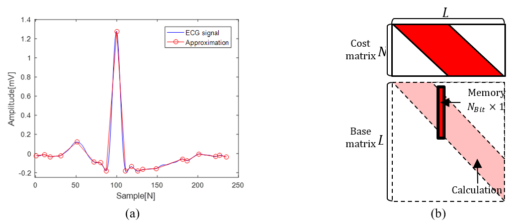
Because the normal beat of the ECG signal repeatedly appears in a shape similar to that of the template, a similar result appears when approximating with the same number of vertices. Therefore, when the vertices’ position information is expressed as a time difference with a vertex corresponding to the template rather than a time difference between vertices, it can be expressed with a relatively low number of data bits.
4.2 Margin of Local Optimization
In general, the time difference between the vertices of the existing approximation has a value of approximately 1 to 32, so a five-bit memory size is required. In contrast, when the time difference with the template vertex is used, most of the error distributions have a value of –3 to +3. Based on this, if the margin for the time difference with the template vertex is given, the amount of location information data is significantly reduced. Fig. 13 shows the reduction of the base matrix’s calculation area when the margin M is given based on each vertex of the template.
Fig. 13.
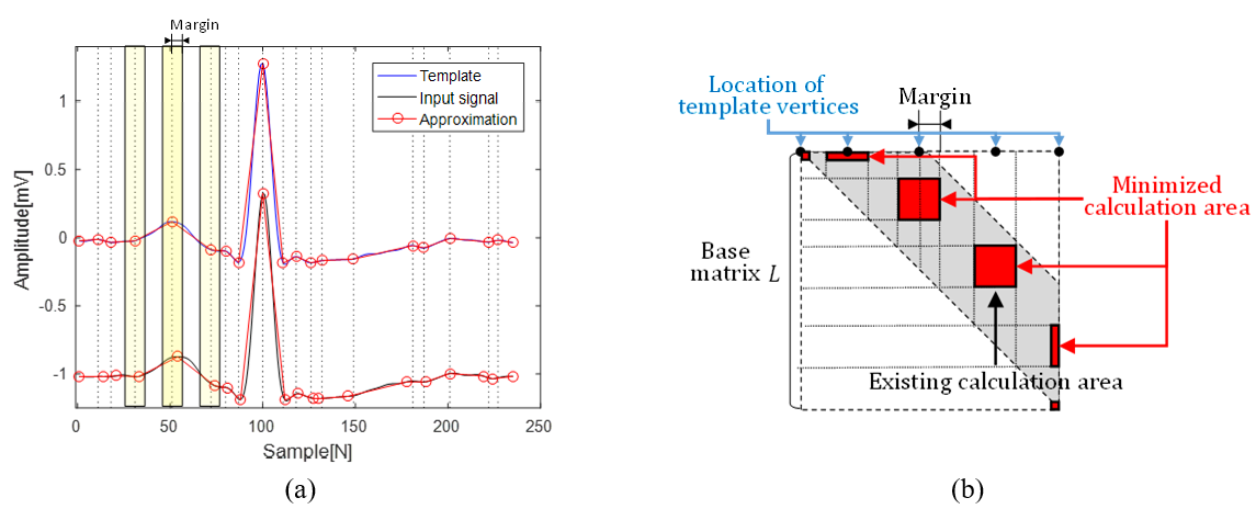
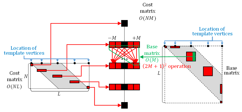
In Fig. 13(b), the existing approximation calculates within a trapezoidal area, but when the template vertices are used, only the inside of the red rectangular areas within the margin range centered on the template’s vertices is calculated, significantly reducing the required calculation. The same is true for the cost matrix. The cost matrix appears as shown in Fig. 14 because it requires calculating values for the [TeX:] $$\pm M$$ area around the template vertices for each row.
Thus, the computation range of cost matrix C(k,j) is limited by the kth vertex of template [TeX:] $$v_{k}^{T}$$ and margin M, as in Eq. (6).
(6)
[TeX:] $$C(k, j)=\min _{v_{k}^{T}-M \leq v_{k} \leq v_{k}^{T}+M}\left(C\left(k-1, v_{k}\right)+C_{0}^{j}\left(v_{k}-\left(v_{k}^{T}-M\right)+1\right)\right)$$In this paper, because [TeX:] $$N_{B i t}$$ and M are given as [TeX:] $$2^{5}=32$$ and 3, respectively, the computation range is significantly reduced.
Fig. 14.

4.3 Optimization of the Algorithm
If the reduced computational area of the cost matrix is expressed around the template vertex, it can be visualized as shown in Fig. 15.
That is, a cost matrix of size [TeX:] $$N \times L$$ becomes size [TeX:] $$N \times(2 M+1)$$, and the size of the base matrix becomes 2M+1. In this way, when the margin is used around the template’s vertices, the memory usage of the cost and base matrices is significantly reduced, and the reduction in the computational area accordingly results in lower processing time. The component of the arranged cost matrix is calculated as in Eq. (7):
(7)
[TeX:] $$C(k, j)=\min _{1 \leq v_{k}^{\prime} \leq 2 M+1}\left(C\left(k-1, v_{k}^{\prime}\right)+C_{0}^{j}\left(v_{k}^{\prime}\right)\right),$$where [TeX:] $$v_{k}^{\prime}=v_{k}-\left(v_{k}^{T}-M\right)+1.$$
As shown in Fig. 15, the spatial complexities of the cost and base matrices are reduced to O(NM) and [TeX:] $$O(M \times 1) \text { from } O(N L) \text { and } O\left(N_{B i t} \times 1\right),$$ respectively.
5. Experiment and Application
5.1 Experimental Results
An experiment was conducted using data from MIT-BIH ADB. Each recording was measured for 30 minutes at a sampling frequency of 360 Hz. Each beat was acquired from 275 ms before to 375 ms after the R-peak. Linear approximation was applied to create 20 vertices for each beat. Because the proposed method is a global optimization method, the template decision and approximation results are almost independent of the processing time. Therefore, after selecting an arbitrary normal beat as a template, the proposed algorithm’s execution time is measured based on a linear approximation of the template.
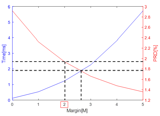
As the size of the margin decreases, the execution time decreases because the operation area decreases, but the approximation error increases. Conversely, as the margin’s size increases, the execution time increases, but the approximation error decreases. A typical method of measuring the signal-approximation error is PRD. The PRD for the input signal X and the approximation signal Y of a signal of length L is calculated according to Eq. (8):
(8)
[TeX:] $$\operatorname{PRD}(X, Y)=100 \% \times \sqrt{\frac{\sum_{i=1}^{L}(X(i)-Y(i))^{2}}{\sum_{i=1}^{L} X^{2}(i)}}.$$Fig. 16 shows the correlation between the PRD and execution time according to the size of the margin.
The execution time and PRD show a nonlinear increase and decrease, respectively. In this case, the intersection of the two graphs is generally evaluated as having the most stable performance. Because the margin has an integer value and this paper focuses on reducing processing time, we analyzed the detailed results when the margin is 2.
First, Fig. 17 shows the distribution of the processing time for each beat when the existing and proposed linear approximation methods are applied. The proposed method improved the execution time by about 12.45 times, from 18.18 ms to 1.46 ms on average.
Fig. 17.
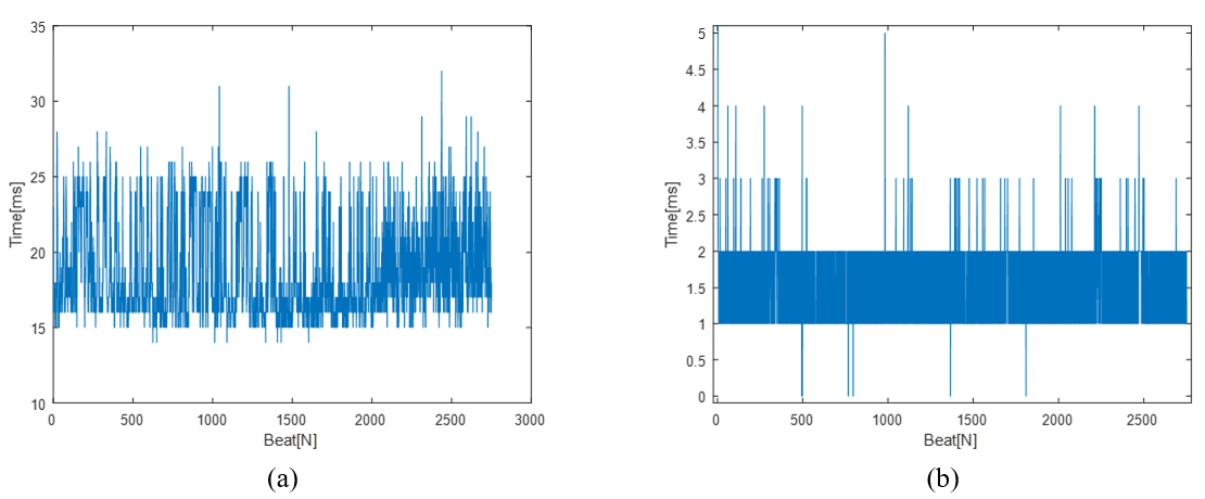
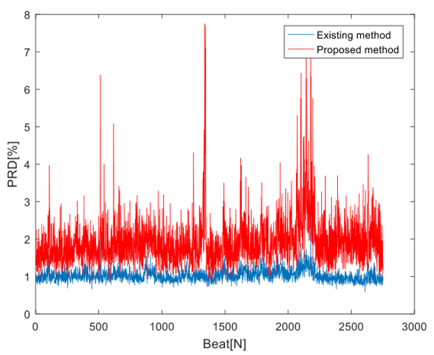
Fig. 18 shows the distribution of the approximation error of each beat based on the linear approximation results. In general, the quality of the PRD is rated as very good (0%–2%) or good (2%–9%) [25]. The existing linear approximation method has a very good approximation error (within 2%). The proposed method has a significantly higher approximation error than the existing method, but it is still good. Although the overall approximation error was higher, 1,756 beats had an approximation error within 2%, and the remaining 995 beats had an approximation error within 9%, so the performance remained consistent.
5.2 Further Applications for the Algorithms
5.2.1 Abnormal beat detection
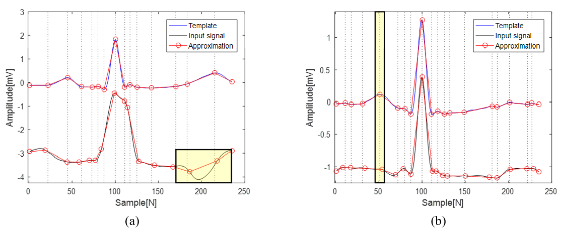
Using the proposed method, approximations are applied based on the template vertices. One problem in the case of an abnormal beat in which the shape information does not match the template is that the approximation is not normally performed due to the margin. Fig. 19 shows an example in which a large approximation error occurs and the approximation error is small, but the feature values are distorted, such as the amplitude of the vertex and the angle with the neighboring vertex.
The proposed method can be used to detect abnormal beats through analysis of the feature values of the vertex and the approximation error.
Fig. 19.
5.2.2 Signal compression with a scaled template
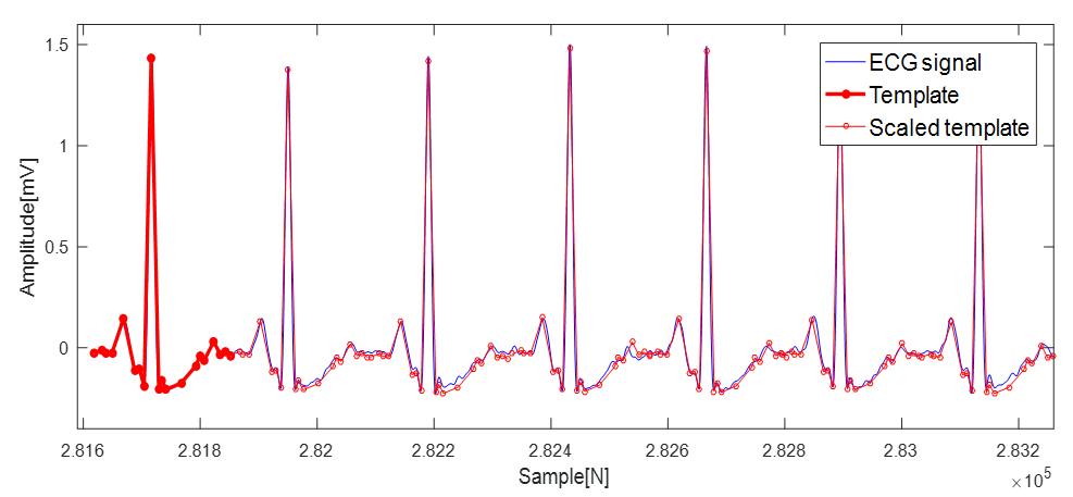
In this paper, the local approximation method uses template vertices because most normal beats have a similar shape. It can be expected that the signal-compression efficiency can be significantly improved by setting the margin to 0 to represent a signal using only the vertex of the template.
Fig. 20 shows the result of representing the signal using a template in which scaling is applied to each normal beat.
An approximation error occurs due to the baseline movement and changes in the intervals between waveforms. However, the shape of the signal is well approximated, confirming the possibility of further research on this approach.
6. Conclusion
In this paper, we proposed a method to optimize local linear approximation within a given margin based on the approximate vertices of an ECG signal template. The proposed algorithm is based on the repetition of similar beats in an ECG signal, so the approximation result is similar to the template. In the experiment, although the approximation error was greater than that of the existing linear approximation method, the proposed method had a stable error within 9%, the performance speed improved by 12.45 times, and the spatial complexity decreased from O(NL) to O(NM), all highlighting the proposed algorithm’s value.
In particular, the proposed algorithm is expected to be very useful if applied only to a normal beat and is based on other abnormal-beat-detection algorithms. In addition, the proposed algorithm may be extended to detect abnormal beats, and further improvement of signal-compression performance can be expected using a scaled template. As such, the proposed algorithm created meaningful results in a basic study on signal compression and the detection of abnormal beats using templates.
Acknowledgement
This study was supported by the BK21 FOUR project funded by the Ministry of Education, Korea (No. 4199990113966, 10%), and the Basic Science Research Program through the National Research Foundation of Korea (NRF) funded by the Ministry of Science and ICT (No. NRF-2019R1A2C2005099, 10%), and Ministry of Education (No. NRF-2018R1A6A1A03025109, 10%; No. NRF-2020R1I1A1A0 1072343, 10%), and Institute of Information & communication Technology Planning & Evaluation (IITP) grant funded by the Korea government (MSIT) (No. 2021-0-00944, Metamorphic approach of unstructured validation/verification for analyzing binary code, 60%), and the EDA tool was supported by the IC Design Education Center (IDEC), Korea.
Biography
Seungmin Lee
https://orcid.org/0000-0002-5910-4387He received the B.S. and M.S. degrees in mathematics and the Ph.D. degree in electronics engineering from Kyungpook National University (KNU), Daegu, South Korea, in 2010, 2012, and 2018, respectively. He expanded his research topics to bioinspired signal processing algorithms and electronics systems. He holds a postdoctoral position at School of Electronics and Electrical Engineering in KNU. His research interests include signal processing, image processing, bioinspired signal processing, and compact system implementation.
Biography
Daejin Park
https://orcid.org/0000-0002-5560-873XHe received the B.S. degree in electronics engineering from Kyungpook National University, Daegu, Korea in 2001, the M.S. and Ph.D. degrees in electrical engineering from the Korea Advanced Institute of Science and Technology (KAIST), Daejeon, Korea, in 2003, and 2014, respectively. He was a research engineer in SK Hynix Semiconductor, Samsung Electronics over 12 years from 2003 to 2014, respectively and have worked on designing low-power embedded processors architecture and implementing fully AI-integrated system-on-chip with intelligent embedded software on the custom-designed hardware accelerator, especially for hardware/software tightly-coupled applications, such as smart mobile devices, industrial electronics. He was nominated as one of Presidential Research Fellows 21, Republic of Korea in 2014. Prof. Park is now with School of Electronics and Electrical Engineering and School of Electronics Engineering as full-time associate professor in Kyungpook National University, Daegu, Korea, since 2014. He has published over 180 technical papers and 40 patents.
References
- 1 S. L. Rohit, B. V. Tank, "IoT based health monitoring system using raspberry PI-review," in Proceedings of 2018 2nd International Conference on Inventive Communication and Computational Technologies (ICICCT), Coimbatore, India, 2018;pp. 997-1002. custom:[[[-]]]
- 2 S. A. Elhannachi, N. Benamrane, T. A. Abdelmalik, "Adaptive medical image compression based on lossy and lossless embedded zerotree methods," Journal of Information Processing Systems, vol. 13, no. 1, pp. 40-56, 2017.doi:[[[10.3745/JIPS.02.0052]]]
- 3 H. Rhim, K. Tamine, R. Abassi, D. Sauveron, S. Guemara, "A multi-hop graph-based approach for an energy-efficient routing protocol in wireless sensor networks," Human-centric Computing and Information Sciences, vol. 8, no. 30, 2018.doi:[[[10.1186/s13673-018-0153-6]]]
- 4 Y. Meng, S. H. Yi, H. C. Kim, "Health and wellness monitoring using intelligent sensing technique," Journal of Information Processing Systems, vol. 15, no. 3, pp. 478-491, 2019.custom:[[[-]]]
- 5 W. M. Kang, S. Y. Moon, J. H. Park, "An enhanced security framework for home appliances in smart home," Human-centric Computing and Information Sciences, vol. 7, no. 6, 2017.doi:[[[10.1186/s13673-017-0087-4]]]
- 6 W. Lee, N. Kim, B. D. Lee, "An adaptive transmission power control algorithm for wearable healthcare systems based on variations in the body conditions," Journal of Information Processing Systems, vol. 15, no. 3, pp. 593-603, 2019.custom:[[[-]]]
- 7 T. Teraoka, "Organization and exploration of heterogeneous personal data collected in daily life," Human-Centric Computing and Information Sciences2012, vol. 2, no. 1, 1962.doi:[[[10.1186/2192--2-1]]]
- 8 T. H. Kim, S. Y. Kim, J. H. Kim, B. J. Yun, K. H. Park, "Curvature based ECG signal compression for effective communication on WPAN," Journal of Communications and Networks, vol. 14, no. 1, pp. 21-26, 2012.doi:[[[10.1109/JCN.2012.6184547]]]
- 9 H. Mamaghanian, N. Khaled, D. Atienza, P. Vandergheynst, "Compressed sensing for real-time energy-efficient ECG compression on wireless body sensor nodes," IEEE Transactions on Biomedical Engineering, vol. 58, no. 9, pp. 2456-2466, 2011.doi:[[[10.1109/TBME.2011.2156795]]]
- 10 R. Bellman, S. Dreyfus, Applied Dynamic Programming, NJ: Princeton University Press, Princeton, 2015.custom:[[[-]]]
- 11 S. Lee, Y. Jeong, D. Park, B. J. Yun, K. H. Park, "Efficient fiducial point detection of ECG QRS complex based on polygonal approximation," Sensors, vol. 18, no. 12, 2018.doi:[[[10.3390/s18124502]]]
- 12 S. Lee, Y. Jeong, J. Kwak, D. Park, K. H. Park, "Advanced real-time dynamic programming in the polygonal approximation of ECG signals for a lightweight embedded device," IEEE Access, vol. 7, pp. 162850-162861, 2019.custom:[[[-]]]
- 13 S. Lee, D. Park, "Enhanced dynamic programming for polygonal approximation of ECG signals," in Proceedings of 2020 IEEE 2nd Global Conference on Life Sciences and Technologies (LifeTech), Kyoto, Japan, 2020;pp. 121-122. custom:[[[-]]]
- 14 M. S. Manikandan, S. Dandapat, "Quality controlled wavelet compression of ECG signals by WEDD," in Proceedings of International Conference on Computational Intelligence and Multimedia Applications (ICCIMA), Sivakasi, India, 2007;pp. 581-586. custom:[[[-]]]
- 15 G. B. Moody, R. G. Mark, "The MIT-BIH arrhythmia database on CD-ROM and software for use with it," in Proceedings of Computers Cardiology Conference, Chicago, IL, 1990;pp. 185-188. custom:[[[-]]]
- 16 M. Merone, P. Soda, M. Sansone, C. Sansone, "ECG databases for biometric systems: a systematic review," Expert Systems with Applications, vol. 67, pp. 189-202, 2017.doi:[[[10.1016/j.eswa.2016.09.030]]]
- 17 F. A. Elhaj, N. Salim, A. R. Harris, T. T. Swee, T. Ahmed, "Arrhythmia recognition and classification using combined linear and nonlinear features of ECG signals," Computer Methods and Programs in Biomedicine, vol. 127, pp. 52-63, 2016.doi:[[[10.1016/j.cmpb.2015.12.024]]]
- 18 G. M. Friesen, T. C. Jannett, M. A. Jadallah, S. L. Yates, S. R. Quint, H. T. Nagle, "A comparison of the noise sensitivity of nine QRS detection algorithms," IEEE Transactions on Biomedical Engineering, vol. 37, no. 1, pp. 85-98, 1990.custom:[[[-]]]
- 19 S. K. Berkaya, A. K. Uysal, E. S. Gunal, S. Ergin, S. Gunal, M. B. Gulmezoglu, "A survey on ECG analysis," Biomedical Signal Processing and Control, vol. 43, pp. 216-235, 2018.doi:[[[10.1016/j.bspc.2018.03.003]]]
- 20 A. P. James, "Heart rate monitoring using human speech spectral features," Human-centric Computing and Information Sciences, vol. 5, no. 30, 2015.doi:[[[10.1186/s13673-015-0052-z]]]
- 21 J. Pan, W. J. Tompkins, "A real-time QRS detection algorithm," IEEE Transactions on Biomedical Engineering, vol. 32, no. 3, pp. 230-236, 1985.doi:[[[10.1109/tbme.1985.325532]]]
- 22 A. Li, S. Wang, H. Zheng, L. Ji, J. Wu, "A novel abnormal ECG beats detection method," in Proceedings of 2010 The 2nd International Conference on Computer and Automation Engineering (ICCAE), Singapore, 2010;pp. 47-51. custom:[[[-]]]
- 23 F. Mokhtarian, R. Suomela, IEEE Transactions on Pattern Analysis and Machine Intelligence, vol, 20, no. 12, pp. 1376-1381, 1998.custom:[[[-]]]
- 24 K. J. O'Connell, "Object-adaptive vertex-based shape coding method," IEEE Transactions on Circuits and Systems for Video Technology, vol. 7, no. 1, pp. 251-255, 1997.doi:[[[10.1109/76.554440]]]
- 25 Y. Zigel, A. Cohen, A. Katz, "The weighted diagnostic distortion (WDD) measure for ECG signal compression," IEEE Transactions on Biomedical Engineering, vol. 47, no. 11, pp. 1422-1430, 2000.custom:[[[-]]]

