Zhang Cheng* and Nanni Huang*
Risk Assessment and Decision-Making of a Listed Enterprise’s L/C Settlement Based on Fuzzy Probability and Bayesian Game Theory
Abstract: Letter of Credit (L/C) is currently a very popular international settlement method frequently used in international trade processes amongst countries around the globe. Compared with other international settlement methods, however, L/C has some obvious shortcomings. Firstly, it is not easy to use due to the sophisticated processes its usage involves. Secondly, it is sometimes accompanied by a few risks and some uncertainty. Thus, highly efficient methods need to be used to assess and control these risks. To begin with, FAHP and KMV methods are used to resolve the problem of incomplete information associated with L/C and then, on this basis, Bayesian game theory is used in order to make more scientific and reasonable decisions with respect to international trade.
Keywords: Bayesian Game Theory , Fuzzy Probability , Listed Enterprise , L/C Settlement
1. Introduction
International trade exchange activities have been taking place in China since the Han Dynasty, 2100 years ago. The Letter of Credit (L/C) itself has been employed in modern financial systems for 130 years and plays a special and irreplaceable role in the international trade settlement process. L/C is often used since it solves one of the most common problems: buyers and sellers inherently live in different countries and, therefore, the information they exchange during international trade transactions is always incomplete and asymmetric. In other words, it is not so easy for buyers to know the sellers’ information thoroughly; and similarly, it is also very difficult for sellers to have full knowledge of the buyers’ information. Thus, it almost impossible for the two parties to trade with each other without any risks, and L/C can only solve such risk problems to some extent.
L/C is widely used around the world. Data shows that 15% or so of international deals are settled with L/C at present, the total amounting to a value of about one million billion US dollars each year. Table 1 shows L/C’s usage percentages in different regions: Asia, about 46%; the Middle East, the highest, about 52%; Africa, the second highest, 49%; and the European Union, the least, making up just 10% [1].
Table 1.
| Region | L/C usage in different regions (%) |
|---|---|
| European Union | 9 |
| The Rest of Europe | 20 |
| North America | 11 |
| Latin America | 27 |
| Middle East | 52 |
| Asia-Pacific | 43 |
| Africa | 49 |
| Asia | 46 |
| Australia and New Zealand | 17 |
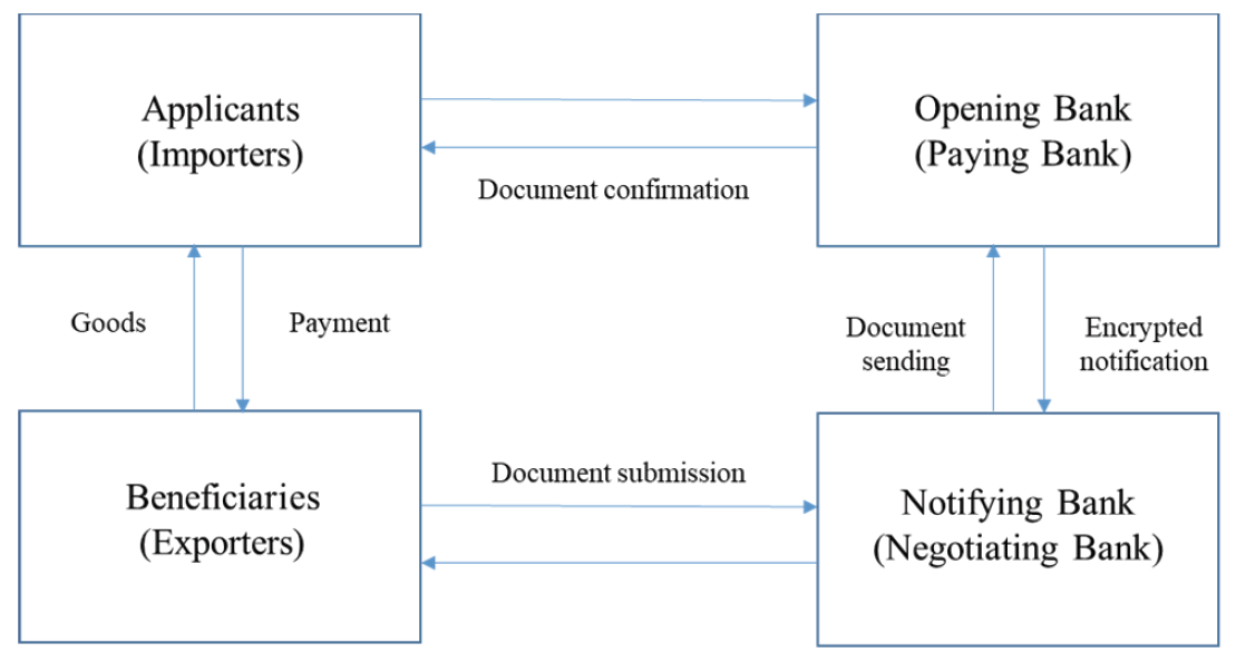
However, L/C does not provide 100% perfect certainty. It also has a few flaws in its usage process. For instance, during the L/C settlement process, there can be many problems, such as L/C soft terms default phenomenon, hard term default phenomenon, invoice default phenomenon, counterfeit L/C phenomenon, and counterfeit bill of loading phenomenon, etc. One report shows that the Chinese Communication Construction Corporation faced a total loss of 250 million Yuan owing to L/C defaults from 2007 to 2008 [2]. Similarly, Chinese banks repay more than 1 billion US dollars to enterprises each year due to malicious international L/C settlement defaults (Fig. 1).
2. Feasibility of Game Theory in the Decision-Making Process against L/C Settlement Risks
Generally, there are two types of export enterprises. One is the listed enterprise and the other is the non-listed enterprise. The risks of L/C with respect to the former will be mainly discussed in the following section.
The Bayesian method can be used to calculate the posterior probability [3]. Firstly, suppose [TeX:] $$\mathrm{p}\left(g_{i}\right)$$ as the prior probability of the participant [TeX:] $$g_{i}, \text { and } \mathrm{p}\left(h_{i}\right)$$ as the probability of new information obtained after investigation [TeX:] $$h_{j}.$$ The conditional probability is then [TeX:] $$\mathrm{p}\left(h_{j} / g_{i}\right).$$ Therefore, the posterior probability [TeX:] $$\mathrm{p}\left(g_{i} / h_{j}\right)$$ can then be easily calculated with the Bayesian formula, if [TeX:] $$\mathrm{p}\left(g_{i}\right), \mathrm{p}\left(h_{i}\right), \mathrm{p}\left(h_{j} / g_{i}\right)$$ is first worked out [4].
(1)
[TeX:] $$\mathrm{P}\left(g_{i} / h_{j}\right)=\left[\mathrm{P}\left(h_{j} / g_{i}\right) \times \mathrm{p}\left(g_{i}\right)\right] / \mathrm{p}\left(h_{j}\right)=\left[\mathrm{P}\left(h_{j} / g_{i}\right) \times \mathrm{p}\left(g_{i}\right)\right] / \sum \mathrm{P}\left(h_{j} / \mathrm{g}_{\mathrm{i}}\right) \times \mathrm{p}\left(g_{i}\right)$$3. Model Assumptions and Design
Firstly, the assumptions of the model are as follows:
(1) International trade markets are fully competitive, and trade parties have the full freedom to buy and sell.
(2) All the trade participants are rational, and they all want to make maximal profit.
(3) There is no non-tariff barrier (technical trade barriers or quota restriction, etc.) between two parties involved in international trade markets.
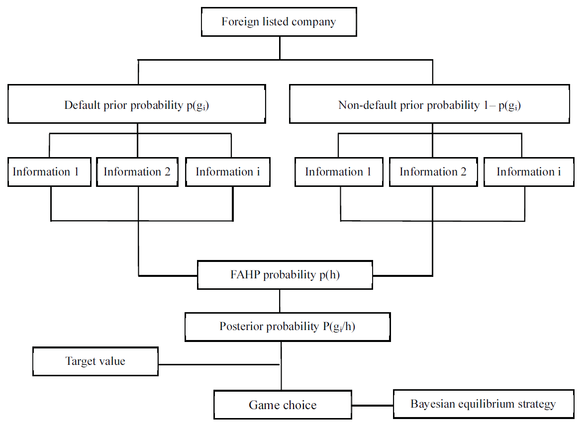
(4) Asset data, the balance sheets and so on in the listed company’s report should be credible. The design model is then as follows (Fig. 2).
3.1 Prior Probability p(gi) of L/C Default by Foreign Listed Enterprise
By analyzing the historical data of foreign export enterprises, we know that:
For instance, suppose the total number of L/C settlements between Chinese enterprises and foreign listed enterprises is n = 1000 times within twenty years, and the total number of L/C defaults by foreign listed enterprises is m = 50 times within twenty years, then the prior probability of L/C usage default can be calculated by the following function:
3.2 Fuzzy Probability P(hj/gi) of L/C Default by Foreign Listed Enterprise
Owing to incomplete information with respect to international trade, fuzzy probability P(hj/gi) is a substitute for accurate probability.
Generally, the factors related to fuzzy probability [TeX:] $$\mathrm{P}\left(h_{j} / g_{i}\right)$$ assessment include: (1) the national risk probability; (2) financial and operational conditions of the listed enterprise itself; (3) soft term risks of the L/C; (4) hard term risks of the L/C; (5) operational risks of banks [5-9].
Among them, factors (1) and (2) are quantitative factors of which the risk probability can be determined through the calculation of data; however, factors (3), (4) and (5) are qualitative factors and their risk probabilities need to be worked out by means of fuzzy comprehensive assessment.
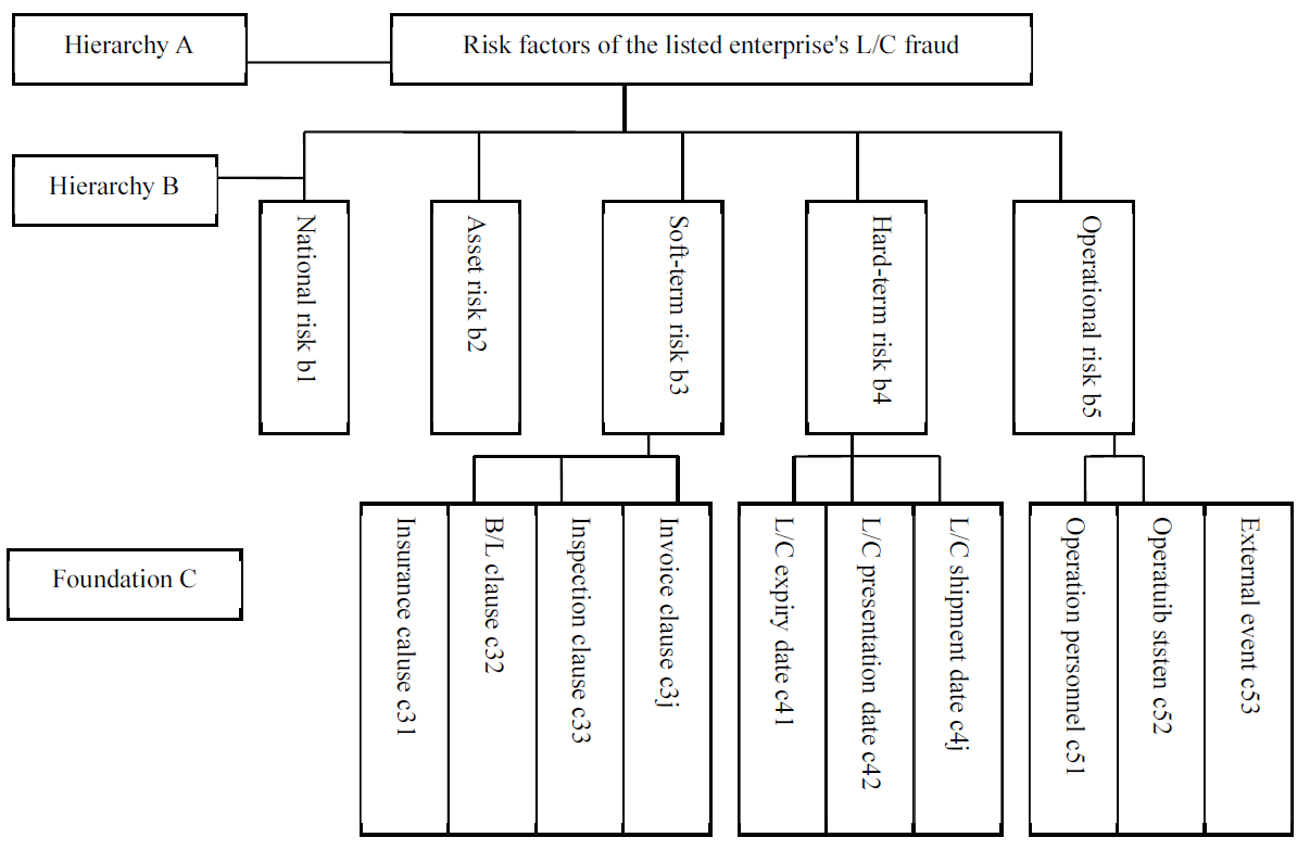
First, set up the analytic hierarchy structure as follows (Fig. 3).
Second, calculate the factor weight [TeX:] $$w_{i j}$$ of all the levels.
Third, get the national risk probability [TeX:] $$\mathrm{P}\left(h_{1} / g_{1}\right)$$ provided by credit rating agencies.
Fourth, calculate the asset risk probability [TeX:] $$\mathrm{P}\left(h_{2} / g_{2}\right)$$ with B-S-M models.
Fifth, find out the fuzzy probability [TeX:] $$\mathrm{P}\left(h_{3} / g_{3}\right)$$ of all the qualitative factors.
And finally, calculate the fuzzy probability of the listed enterprise’s L/C default:
(3)
[TeX:] $$\mathrm{P}\left(h_{j} / g_{i}\right)=\sum w_{i j} \times \mathrm{P}\left(h_{j} / g_{i}\right)$$3.2.1 National risk probability [TeX:] $$\mathrm{P}\left(h_{j} / g_{i}\right)$$ of the foreign listed enterprise
National risk probability refers to the probability of international trade risks, international finance risks as well as international investment risks influenced by factors such as a country’s political, cultural, economic, military, diplomatic, and social environments.
Nowadays, government departments and credit rating agencies in many countries such as the United States, China and Switzerland release annual reports of their country’s national risk. These reports reveal to people how investment and trade risks are distributed all over the world. Table 2 shows the relationship between the American financial service, Standard and Poor’s sovereign credit rating and the default probability of national risk [10].
For example, China’s sovereign credit rating is A+, so we learn from the table that the median value of its national risk default probability is 0.06%. Nigeria’s sovereign credit rating is B+, and by looking it up in Table 2, we learn that the median value of its national risk default probability is 3.00%.
Table 2.
| Rating | SP’s rating | Expected default probability (%) | ||
|---|---|---|---|---|
| Upper limit | Lower limit | Median | ||
| 1 | [TeX:] $$\mathrm{AAA} / \mathrm{AA}^{+}$$ | 0.02 | 0 | 0.01 |
| 2 | [TeX:] $$\mathrm{AA} / \mathrm{A}^{-}$$ | 0.04 | 0.02 | 0.03 |
| … | … | … | … | … |
| 13 | [TeX:] $$\mathrm{B}^{+}$$ | 3.50 | 2.50 | 3.00 |
| 17 | [TeX:] $$\leq C C C$$ | 100.00 | 10.00 | 20.00 |
3.2.2 Asset risk probability [TeX:] $$\mathrm{P}\left(h_{2} / g_{2}\right)$$ of the foreign listed enterprise
Based on the listed enterprise’s information disclosure principle, we can obtain an enterprise’s default probability through the KMV model, which is an improvement on the Black–Scholes–Merton (B–S–M) pricing option.
In the B–S–M model, E = market price per share, D = the debt value per share, [TeX:] $$\mathrm{V}_{0}=$$ the asset value per share, T = the time of the share, r = the non-risk interest rate, and [TeX:] $$\sigma_{0}=$$ the variation of the asset value wave.
The parameters of the above formula are:
(5)
[TeX:] $$d_{1}=\left[\ln \left(V_{0} / D\right)+\left(r+0+5 \sigma_{0}^{2}\right) \cdot T\right] /\left(\sigma_{0} \cdot \sqrt{T}\right)$$
Owing to the fact that the computer languages, MATLAB, Python, C and R are inaccessible to the average nonprofessional, we may use the simulation model [11] designed by myself to calculate out [TeX:] $$V_{0}$$ and [TeX:] $$\sigma_{0}$$ very easily:
(1) Find out the listed enterprise’s default point DPT. For example,
where CL is current loan and LL is long loan.
(2) Calculate the listed enterprise’s distance-to-default (DD) [11].
Calculate the default probability according to the function [TeX:] $$\mathrm{DD}: \mathrm{EDF}=\mathrm{p}\left(V_{0}<\mathrm{DPT}\right).$$ And here, [TeX:] $$V_{0}$$ stands for the enterprise’s asset value.
3.2.3 Fuzzy risk probability p(h3/g3) of L/C’s soft terms, hard terms and operational risk
Fuzzy method is a mathematical method attempting to solve problems by setting values to an imprecise spectrum of data in order to arrive at the most possible accurate conclusion [12].
Hard terms: these are the terms of the applicants and beneficiaries, the expiry date, shipment date, shipment port, the unloading port, presentation period, the negotiating and the issuing bank, etc., all of which are highly necessary parts of all L/Cs.
Soft terms or soft clauses are of two kinds: the non-purpose default terms, and other risky clauses set by the applicant with the purpose of malignant default [13,14].
Operational risk: Operational risk is caused by imperfect or defective internal procedures, personnel or external events.
(1) Set up the fuzzy set
[TeX:] $$\mathrm{F}_{1}=\left(\mathrm{C}_{21}, \mathrm{C}_{22}, \ldots \mathrm{C}_{2 \mathrm{n}}\right)=$$ (insurance clauses, B/L clauses, inspection terms, invoice terms…)
[TeX:] $$\mathrm{F}_{2}=\left(\mathrm{C}_{21}, \mathrm{C}_{22}, \ldots \mathrm{C}_{2 \mathrm{n}}\right)=$$ (goods delivery risk, financial risk, and settlement method risk...)
[TeX:] $$\mathrm{F}_{3}=\left(\mathrm{C}_{31}, \mathrm{C}_{32}, \ldots \mathrm{C}_{5 \mathrm{n}}\right)=$$ (operator risk, the operating system risk...)
[TeX:] $$\mathrm{F}=\left(\mathrm{F}_{1}, \mathrm{F}_{2}, \mathrm{F}_{3}, \mathrm{F}_{4}, \mathrm{F}_{5}\right)$$
(2) Set up the fuzzy comment set V
Multi-level comment sets can be set up in accordance with the actual conditions.
V = {Super big risk probability, big risk probability, average risk probability, small risk probability, super small risk probability}
(3) Inquire with related experts to assess these L/C information by comment set V.
For example, in the following table, the membership grades of the column i and the line j is unit [TeX:] $$B_{i j}:$$
(8)
[TeX:] $$V_{1}=\begin{array}{c|ccccc} & \text { Super big risk } & \text { Big risk } & \text { Average risk } & \text { Small risk } & \text { Super small risk } \\ \hline \text { Insurance clauses } & \mathrm{B}_{11} & \mathrm{B}_{12} & \mathrm{B}_{13} & \mathrm{B}_{14} & \mathrm{B}_{15} \\ \mathrm{B} / \mathrm{L} \text { clauses } & \mathrm{B}_{21} & \mathrm{B}_{22} & \mathrm{B}_{23} & \mathrm{B}_{24} & \mathrm{B}_{25} \\ \text { Inspection terms } & \mathrm{B}_{31} & \mathrm{B}_{32} & \mathrm{B}_{33} & \mathrm{B}_{34} & \mathrm{B}_{35} \\ \text { Invoice terms } & \mathrm{B}_{41} & \mathrm{B}_{42} & \mathrm{B}_{43} & \mathrm{B}_{44} & \mathrm{B}_{45} \\ \ldots & \mathrm{B}_{\mathrm{n} 1} & \mathrm{B}_{\mathrm{n} 2} & \mathrm{B}_{\mathrm{n} 3} & \mathrm{B}_{\mathrm{n} 4} & \mathrm{B}_{\mathrm{n} 5} \end{array}$$Similarly the fuzzy set [TeX:] $$\mathrm{V}_{2}, \mathrm{V}_{3}, \mathrm{V}_{4}, \mathrm{V}_{5}$$ can be set up.
Fuzzy comprehensive assessment:
[TeX:] $$\mathrm{A}=\mathrm{W}_{\mathrm{c}} \times \mathrm{V}_{\mathrm{i}}^{\mathrm{T}}=\left(\mathrm{W}_{\mathrm{c} 1}, \mathrm{W}_{\mathrm{c} 2}, \mathrm{W}_{\mathrm{c} 3}, \ldots \mathrm{W}_{\mathrm{cn}}\right) \times\left(\mathrm{V}_{1}, \mathrm{V}_{2}, \mathrm{V}_{3}, \mathrm{V}_{4}, \mathrm{V}_{5}\right)^{\mathrm{T}}=\left(\mathrm{A}_{1}, \mathrm{A}_{2}, \ldots \ldots \mathrm{A}_{5}\right)$$
For example, [TeX:] $$\mathrm{A}_{1}=\mathrm{W}_{1 \mathrm{c}} \times \mathrm{V}_{1}=\left(\mathrm{W}_{\mathrm{c} 11}, \mathrm{W}_{\mathrm{c} 12}, \mathrm{W}_{\mathrm{c} 1 \mathrm{n}}\right) \times$$
(9)
[TeX:] $$\left[\begin{array}{ccccc} \mathrm{B}_{11} & \mathrm{B}_{12} & \mathrm{B}_{13} & \mathrm{B}_{14} & \mathrm{B}_{15} \\ \mathrm{B}_{21} & \mathrm{B}_{22} & \mathrm{B}_{23} & \mathrm{B}_{24} & \mathrm{B}_{25} \\ \cdots & \cdots & \cdots & \cdots \\ \mathrm{B}_{n 1} & \mathrm{B}_{\mathrm{n} 2} & \mathrm{B}_{\mathrm{n} 3} & \mathrm{B}_{\mathrm{n} 4} & \mathrm{B}_{\mathrm{n} 5} \end{array}\right]$$Similarly [TeX:] $$\mathrm{A}_{2}, \mathrm{A}_{3}, \mathrm{A}_{\mathrm{n}}$$ can be worked out.
(4) Calculate the fuzzy probability for the listed enterprise’s qualitative factors:
[TeX:] $$\mathrm{p}\left(h_{3}\right), \mathrm{p}\left(h_{4}\right), \mathrm{p}\left(h_{5}\right)=\mathrm{w}_{\mathrm{cj}}(\text { weights of factors in foundation } \mathrm{C}) \times\left(\mathrm{A}_{1}, \mathrm{A}_{2}, \ldots \mathrm{A}_{\mathrm{n}}\right)$$
3.2.4 Calculate the comprehensive probability of the listed enterprise’s L/C default risks
(10)
[TeX:] $$\mathrm{P}\left(h_{j} / g_{i}\right)=\sum w_{i j} \times \mathrm{P}\left(h_{j} / g_{i}\right)$$where [TeX:] $$\mathrm{Wij}$$ is the weight and [TeX:] $$\mathrm{p}\left(h_{j}\right)$$ is its probability.
4. Calculation of the Posteriori Probability based on the Bayesian Formula
According to the Bayesian formula:
(11)
[TeX:] $$\mathrm{P}\left(g_{i} / h_{j}\right)=\left[\mathrm{P}\left(h_{j} / g_{i}\right) \times \mathrm{p}\left(g_{i}\right)\right] / \mathrm{p}\left(h_{j}\right)=\left[\mathrm{P}\left(h_{j} / g_{i}\right) \times \mathrm{p}\left(g_{i}\right)\right] / \sum w_{i j} \times \mathrm{p}\left(h_{j}\right)$$[TeX:] $$\mathrm{p}\left(h_{j}\right)$$ always may be considered as trending to 1 by international trade experts.
5. Game Decision-Making and the Bayesian Nash Equilibrium
6. Case Study
5.1 Model Assumptions
(1) Trade term, CIF; the insurance fee, S
(2) The posteriori probability of the L/C risk: [TeX:] $$\mathrm{P}\left(g_{i} / h_{j}\right)=\mathrm{P}_{0}$$
(3) The cost for issuing the L/C, [TeX:] $$\mathrm{F}_{1}$$
(4) The price of the commodity for exporters, P; the quantity, Q; and the cost, X
(5) The sale price of the importer, [TeX:] $$P^{+};$$ the cost of the sale, [TeX:] $$\mathrm{X}^{+}$$
(8) Total expense of shipment, [TeX:] $$\mathrm{F}_{2}$$
(9) The negotiation time for the L/C: t, months; the month discount rate, r
5.2 Hypothesis 1: The Importer Does Not Default and The Exporter Accepts
The exporter’s total revenue will be:
The exporter’s total revenue will be 0.
5.3 Hypothesis 2: The Importer Does Not Default and The Exporter Refuses
The importer’s total revenue will be:
The importer’s total revenue becomes 0.
5.4 Hypothesis 3: The Importer Defaults and The Exporter Refuses
The exporter's total loss will be:
The exporter's total revenue will be:
5.5 Hypothesis 4: The Importer Defaults and The Exporter Accepts
Under this condition, suppose the exporter’s loss is y%, then the importer’s total revenue will be:
(16)
[TeX:] $$\pi^{5}=\pi^{4}+\mathrm{y} \% \times \mathrm{PQ}=\mathrm{P}^{+} \times \mathrm{Q}+\mathrm{P}(1-\mathrm{y} \%) \times \mathrm{Q}-\mathrm{X}^{+}$$The importer’s total loss will be the one side shipment cost:
5.6 Therefore, The Importer's Balance Point
That is,
5.7 All Above Conditions can be Described in the Game Theory [15] (Table 3)
Table 3.
| Importer | |||
|---|---|---|---|
| No default [TeX:] $$\left(1-P_{\theta}^{\sim}\right)$$ | Default [TeX:] $$P_{0}$$ | ||
| Exporter | Accept | [TeX:] $$\pi^{l}, \pi^{4}$$ | [TeX:] $$\pi^{1}-y \% \times P Q, \pi^{4}+y \% \times P Q$$ |
| Refuse | 0, 0 | [TeX:] $$-\left(2 \times F_{2}+S\right),-F_{1}$$ | |
Therefore, if the value of the comprehensive risk assessment of the L/C is [TeX:] $$\mathrm{P}_{0}^{\wedge},$$ then the exporter’s expectation value [TeX:] $$\mathrm{E}_{1}$$ will be:
(20)
[TeX:] $$E_{1}=\left(1-\mathrm{P}_{0}^{\sim}\right) \pi^{l}+P_{0}^{\sim} \times\left(\pi^{l}-y \% \times P Q\right)=\pi^{1}-P_{0}^{\sim} \times y \% \times P Q$$when [TeX:] $$\mathrm{E}_{1}>0,$$
(21)
[TeX:] $$P_{0}^{\sim}<\pi^{l} / y \% \times P Q=e\left\{P \times Q-\left(F_{2}+S\right)-X\right\} /(1+r)^{t} y \% \times P Q$$And, in accordance with Eq. (17): [TeX:] $$\mathrm{y} \% \times \mathrm{PQ}<-\pi^{2}=2 \times \mathrm{F}_{2}+\mathrm{S},$$ the following result is achieved:
(22)
[TeX:] $$P_{0}<\left\{P \times Q-\left(F_{2}+S\right)-X\right\} /(1+\mathrm{r})^{t}\left(2 \times \mathrm{F}_{2}+\mathrm{S}\right)$$That is to say, the exporter will consider accepting this L/C only under condition (22) being achieved and arranging the shipment accordingly.
In September 2005, one company purchased 20 tons of mono ammonium phosphate from Chengdu Chuanke Chemical Co. Ltd. with the price of one FCL being $585.00/MT using mutually agreed CIF trade terms. The destination port was the Nhava Sheva Port, India. The ocean freight cost was $200.00/FCL. The production cost of ammonium phosphate mono in Chengdu Chuanke Chemical Co. Ltd. was $300/MT. The negotiation time was three months, and the interest rate was r = 1.2%. The insurance premium was $50.00.
According to above information, Chengdu Chuanke Chemical Co. Ltd. faced the following game conditions:
1. If calculated with (3), (4), (5), (6), (7), (8), and (9), then [TeX:] $$\mathrm{p}\left(g_{i}\right)=0.4, \mathrm{p}\left(h_{j} / g_{i}\right)=0.75, \text { and } \mathrm{p}\left(h_{j}\right)=\Sigma w_{i j} \times \mathrm{p}\left(h_{j}\right) \approx 1.$$ Then using the Bayesian method, Chengdu Chuanke Chemical Co. Ltd. worked out the default posterior probability of the India Enterprise as 0.3 by formula (10) as follows:
(23)
[TeX:] $$\mathrm{P}\left(g_{i} / h_{j}\right)=\left[\mathrm{P}\left(h_{j} / g_{i}\right) \times \mathrm{p}\left(g_{i}\right)\right] / \mathrm{p}\left(h_{j}\right)=\left[\mathrm{P}\left(h_{j} / g_{i}\right) \times \mathrm{p}\left(g_{i}\right)\right] / \sum \mathrm{w}_{\mathrm{ij}} \times \mathrm{p}\left(h_{j}\right)=0.4 \times 0.75 \div 1=0.3$$2. After negotiating, the two parties modified four clauses in the L/C . This was calculated out with (3)(4)(5)(6)(7)(8) (9): p(gi)=0.4, [TeX:] $$\mathrm{P}\left(h_{j} / g_{i}\right)=0.015, \text { and } \mathrm{p}\left(h_{j}\right)=\sum w_{i j} \times \mathrm{p}\left(h_{j}\right) \approx 1.$$ The default posterior probability became 0.06 in the second test by formula (10) as follows:
(24)
[TeX:] $$\mathrm{P}\left(g_{i} / h_{j}\right)=\left[\mathrm{P}\left(h_{j} / g_{i}\right) \times \mathrm{p}\left(g_{i}\right)\right] / \mathrm{p}\left(h_{j}\right)=\left[\mathrm{P}\left(h_{j} / g_{i}\right) \times \mathrm{p}\left(g_{i}\right)\right] / \sum w_{i j} \times \mathrm{p}\left(h_{j}\right)=0.4 \times 0.015 \div 1=0.06$$3. Price (P)=585; quantity Q=20; time T=3; interest rate R=1.2%; production cost C=300×20=6000; insurance premium cost S=50; freight F2=200.
First, according to the formula (22), only when [TeX:] $$P_{0}^{\sim}<\left\{\mathrm{P} \times \mathrm{Q}-\left(\mathrm{F}_{2}+\mathrm{S}\right)-\mathrm{C}\right\} /(1+\mathrm{r})^{\mathrm{t}}\left(2 \times \mathrm{F}_{2}+\mathrm{S}\right)$$ should Chengdu Chuanke Chemical Co. Ltd. accept this L/C. Then through computation obtained the result.
(25)
[TeX:] $$\left\{P \times Q-\left(F_{2}+S\right)-X\right\} /(1+r)^{t}\left(2 \times F_{2}+S\right)=8.3$$And [TeX:] $$P_{0}=6 \%=0.06,$$ being far smaller than 8.3. That is to say:
(26)
[TeX:] $$P_{0}^{\sim}<\left\{P \times Q-\left(F_{2}+S\right)-X\right\} /(1+r)^{t}\left(2 \times F_{2}+S\right)$$Based on the above two conditions, Chengdu Chuanke Chemical Co. Ltd. believed that the risk of this L/C was quite low, and thus accepted the L/C and submitted all the shipping documents to the issuing bank. The author, as one of the staff in charge, took part in the risk assessment and foreign exchange work of the L/C. The result was consistent with expectations and three months after the shipment, Chengdu Chuanke Chemical Co. Ltd. successfully settled the L/C and obtained the value of the goods in US dollars.
7. Conclusion
With the development of globalization, many companies treat L/C as a relatively safe settlement method. However, the widespread L/C default phenomenon has, in fact, greatly restricted the development of international trade. What is more, previous L/C risk studies, though many, have not really managed to solve the problems by means of judicature, which often merely consumes a lot of enterprises’ time and money. In order to circumvent the risks of L/C in the future, the author has found a relatively scientific and reasonable method for L/C risk assessment and decision-making based on personal experience with international trade practice. It is hoped that yet more useful methods might be provided in later studies.
Biography
Cheng Zhang
https://orcid.org/0000-0002-2003-4174He finished his postdoctoral training at the School of Finance at the Shanghai University of Finance and Economics, and received his doctoral degree at Tongji University’s School of Economics and Management. Currently, he is the Director of Finance at the Department of Economics and Finance, Yangtze Normal University.
Biography
References
- 1 2003;, https://www.scribd.com/document/43959409/lettcredr
- 2 2010 (Online). Available, https://finance.qq.com/a/20100805/001698.htm
- 3 C. Zhang, "The Risk of L/C in International DCM System," Soft Science, vol. 24, no. 2, pp. 60-63, 2010.custom:[[[-]]]
- 4 S. Han, I. Y. Lee, J. H. Ahn, "Two-dimensional joint bayesian method for face verification," Journal of Information Processing Systems, vol. 12, no. 3, pp. 381-391, 2016.doi:[[[10.3745/JIPS.02.0036]]]
- 5 Y. J. Mao, "On the fraudulent conduct of LC and judicial relief," Annual of China Maritime Law, vol. 2006, pp. 186-197, 2006.custom:[[[-]]]
- 6 W. Jiang, "Research on the L/C soft clause protection form a case," Practice in Foreign Economic Relations and Trade, vol. 2018, no. 4, pp. 71-74, 2018.custom:[[[-]]]
- 7 Y. Chen, "The discerning and dealing with methods of L/C soft clauses," Practice in Foreign Economic Relations and Trade, vol. 2016, no. 4, pp. 57-59, 2016.custom:[[[-]]]
- 8 S. Zhang, "The L/C soft clauses protections of e-business in B2B trade," Jiangsu Commercial Forum, vol. 2008, no. 3, pp. 39-41, 2018.custom:[[[-]]]
- 9 Y. Xu, "The dealing with methods of L/C soft clauses," Legal System and Society, vol. 2017, no. 16, pp. 88-89, 2017.custom:[[[-]]]
- 10 https://www.standardandpoors.com/en_US/web/guest/home
- 11 C. Zhang, C. Ke, "Study listed high-tech small and medium companies default risks based on KMV model simulation system in China," Finance and Accounting Monthly, vol. 2017, no. 20, pp. 81-88, 2017.custom:[[[-]]]
- 12 O. P. Verma, V. Jain, R. Gumber, "Simple fuzzy rule based edge detection," Journal of Information Processing Systems, vol. 9, no. 4, pp. 575-591, 2013.doi:[[[10.3745/JIPS.2013.9.4.575]]]
- 13 H. Shi, W. Ni, "The discerning methods of L/C soft clauses," Knowledge Economy, vol. 2017, no. 11, pp. 45-56, 2017.custom:[[[-]]]
- 14 J. Ye, W. Zhou, "The protection ways of L/C soft clauses," China Circulation Economy, vol. 2017, no. 12, pp. 20-21, 2017.custom:[[[-]]]
- 15 W. Zhang, Game Theory and Information Economics, China: Shanghai People's Publishing, Shanghai, 2004.custom:[[[-]]]


