Liping Zhang* , Song Li* , Yingying Guo* and Xiaohong Hao*
A Method for k Nearest Neighbor Query of Line Segment in Obstructed Spaces
Abstract: In order to make up the deficiencies of the existing research results which cannot effectively deal with the nearest neighbor query based on the line segments in obstacle space, the k nearest neighbor query method of line segment in obstacle space is proposed and the STA_OLkNN algorithm under the circumstance of static obstacle data set is put forward. The query process is divided into two stages, including the filtering process and refining process. In the filtration process, according to the properties of the line segment Voronoi diagram, the corresponding pruning rules are proposed and the filtering algorithm is presented. In the refining process, according to the relationship of the position between the line segments, the corresponding distance expression method is put forward and the final result is obtained by comparing the distance. Theoretical research and experimental results show that the proposed algorithm can effectively deal with the problem of k nearest neighbor query of the line segment in the obstacle environment.
Keywords: Line Segment k Nearest Neighbor , Line Segment Obstacle Distance , Line Segment Voronoi Diagram , Nearest Neighbor Query , Spatial Database
1. Introduction
At present, with the rapid development of application fields such as geographic information system, computer-aided design, intelligent identification system, Internet of Things, decision support system, the spatial database query technology has more important significance. The nearest neighbor query [1-3] is one of the foundations of the spatial database query. A new ST-R tree index is designed by [4] and the nearest neighbor query algorithm in accordance with spatio-temporal information is proposed. The authors [5] proposed the nearest neighbor query algorithm in the road network environment by using the characteristics of network Voronoi diagram. The nearest neighbor query method based on random partition tree is proposed in [6]. In recent years, many variants of the nearest neighbor query were derived based on the research of nearest neighbor query, for example, the reverse nearest neighbor query [7,8], the group nearest neighbor query [9,10], the continuous nearest neighbor query [11,12], the nearest neighbor query based on uncertain data [13], the aggregate nearest neighbor query [14], the strong nearest neighbor query [15], and so on.
In reality, some restrictions on geographical are inevitable, the factors of obstacle must be taken into consideration by the shortest distance between two objects. In [16], the nearest neighbor query method is proposed to preserve the location privacy in obstacle space. In [17], the reverse k nearest neighbor query method is put forward, and the search of influence scope of the query space in the obstacle space is realized. The authors [18] proposed a new index structure O-tree, which is used to store the obstacle data, and solved the nearest neighbor query problem in obstacle space. According to the different position relationship of minimum outsourcing distance between the point in the data set and the query set, the authors [19] proposed a new variant nearest neighbor query in an obstacle environment. In [20], the method of the group reverse k nearest neighbor query in obstructed space was proposed. The algorithms in static obstacle environment and dynamic obstacle environment were given respectively.
The above research work mainly focuses on spatial data points, however, in the practical exploration of query problems, if the spatial objects are abstracted into points, the accuracy of the query results will be impacted, such as mountains, rivers, roadblock, and so on. They are not suitable to be abstracted into points in the process. In order to improve the efficiency of the query, some spatial objects can be abstracted as line segments. [21] solved the nearest neighbor problem of line segments for the first time and proposed the concept and the corresponding nearest neighbor query algorithm based on the line segments. [22] required that all the nodes in the SI-tree are ordered by the relation of its geometric position, which makes that the line segment nearest neighbor query can be quickly located the intermediate node. [23] queried the nearest neighbor properties pair by using the nearest neighbor and local dynamic properties of two Voronoi diagrams. By judging the position relationship between the query line segment and the security region, the problem of the moving k nearest neighbor query over the line segments is solved in [24].
For the nearest neighbor query based on the points in obstacle space, if there is an obstacle between the query point and the data point, then the query will surely be affected and it is necessary to calculate the obstacle distance. However, if the query object is abstracted as a line segment, then the query line segment and the data line segment may be completely visible, partly visible and completely invisible. Therefore, the k nearest neighbor query of the line segment in obstacle space is a new problem to be solved in this paper. The method proposed in this paper is widely used in real life. For example, if some people want to buy a house which is nearest to a school, then the effects of other buildings (obstacles) should be taken into consideration when calculating the shortest distance between the school and the buildings. At this point, the k nearest neighbor query of line segment algorithm in obstacle space which is proposed in this paper can be used. Also, during the railway construction, it will inevitably encounter obstacles such as mountains, rivers, and other factors, and in this case, the k nearest neighbor query of line segment algorithm in obstacle space can be used in order to reduce the query error. The main contributions of this paper are as follows:
(1) The new problem of the obstacle k nearest neighbor of line segment query is presented and formalized defined. The role of the query is discussed in detail.
(2) The study of this paper is divided into two stages: the pruning process and the refining process. First, according to the properties of the line segment Voronoi diagram, this paper proposes the pruning rules for data line segments and obstacles, and the corresponding pruning algorithms are given. In the refining process, the methods of expressing obstacle distance are given. Finally, the STA_OLkNN algorithm is proposed. The proposed algorithm can effectively deal with the problem of k nearest neighbor query of the line segment in the obstacle environment.
2. Basic Definitions and Properties
DEFINITION 1 (Line segment Voronoi diagram [25]). Given a set of disjoint adjacent line segments [TeX:] $$L=\left\{l_{1}, \ldots, l_{n}\right\}$$ and end points of each line segment. The line segment Voronoi diagram divided the plane into several connected regions, which is called Voronoi region. Every region is correspond to each line segment. Voronoi diagram region of each generated line segment is given by the equation: [TeX:] $$V L\left(l_{i}\right)=\{p |\left.d\left(p, l_{i}\right) \leq d\left(p, l_{j}\right)\right\},$$ among which [TeX:] $$i \neq j, j \in I_{n}, \text { and } d\left(p, l_{i}\right)$$ are the shortest distance between p and line segment [TeX:] $$l_{i},$$ (linear distance between point p and line segment [TeX:] $$l_{i}$$ in Euclidean space). The region decided by [TeX:] $$l_{i}$$ is called Voronoi polygon. The figure defined by [TeX:] $$V L(L)=\left\{V L\left(l_{1}\right), \ldots, V L\left(l_{n}\right)\right\}$$ is called line segment Voronoi diagram. Each edge of a line segment Voronoi diagram is composed of a straight line segment or a parabola segment. Voronoi polygons which share the same edge are called adjacent polygons, their generated segments are called adjacent generation line segments.
Property 1. The nearest neighbor of generated line segment li is in the adjacent generated line segment of [TeX:] $$l_{i}$$.
DEFINITION 2 (k level adjacent generated line segment [25]). Given a set of generation line segments [TeX:] $$L=\left\{l_{1}, l_{2}, \ldots, l_{n}\right\}$$ in the Voronoi diagram, among which [TeX:] $$2<n<\infty,$$ and when [TeX:] $$i \neq j \text { then } l_{i} \neq l_{j}$$ Among them, i, [TeX:] $$j \in I_{n}=\{1, \ldots, n\}.$$ The k level adjacent generation line segment of [TeX:] $$l_{i}$$ is defined as [TeX:] $$A G_{k}\left(l_{i}\right)=\left\{l_{j} | V L(l) \text { and } V L\left(l_{j}\right)\right.$$ has common edge, [TeX:] $$\left.l \in A G_{k-1}\left(l_{i}\right)\right\}.$$
DEFINITION 3 (Line segment visualization). There are two line segments [TeX:] $$l_{i} \text { and } l_{j}$$ in obstacle environment, we connect the left and right ends of the two line segments to form a polygon P. If P does not intersect with any obstacles, then the line segment [TeX:] $$l_{i} \ and \ l_{j}$$ are completely visible; If there is an obstacle which has intersection with any side of P, then the line segment [TeX:] $$l_{i} \text { and } l_{j}$$ are partly visible; If there is an obstacle which has more than one intersection with P, then the line segment [TeX:] $$l_{i} \text { and } l_{j}$$ are completely invisible.
DEFINITION 4 (Line segment shortest distance [21]). Given two line segment L and K, the point [TeX:] $$l_{j} \in L$$ the point [TeX:] $$k, k_{i}, k_{j} \in K, \text { dist }(l, k)$$ represents the distance from point l to point k, suppose the shortest distance between line L and K is dist(L, K). Then [TeX:] $$\operatorname{dist}(L, K)=\left\{\operatorname{dist}\left(l_{i}, l_{k}\right) | \operatorname{dist}\left(l_{i}, k_{i}\right) \leq \operatorname{dist}\left(l_{j}, k_{j}\right)\right\}.$$
DEFINITION 5 (Nearest distance of line segment with obstacles). There is a query line segment [TeX:] $$l_{q}$$ (suppose its left and right end points are respectively m and n) and data line segment [TeX:] $$l_{i}.$$ If two line segments are visible, the Euclidean distance of two line segments is noted as [TeX:] $$V \operatorname{dist}\left(l_{i}, l_{q}\right),$$ then the obstacle distance of two line segments is equal to the Euclidean distance, that is [TeX:] $$\text {Odist}\left(l_{i}, l_{j}\right)=\operatorname{Vdist}\left(l_{i}, l_{j}\right).$$ If two line segments are completely invisible and there is an effective obstacle [TeX:] $$O_{k}$$ between two line segments, then the obstacle distance is the shortest distance of the two line segments bypass the obstacles, which is [TeX:] $$\left.\left.\text { Odist=min\{ dist(m, }\left.O_{k}\right)+\operatorname{dist}\left(O_{k}, l_{i}\right), \text { dist( } n, O_{k}\right)+\operatorname{dist}\left(O_{k}, l_{i}\right)\right\}.$$
DEFINITION 6 (Obstacle k nearest neighbor of line segment query). Given data line segment set [TeX:] $$L=\left\{l_{1}\right.\left.l_{2}, \ldots, l_{n}\right\}$$ and obstacle set [TeX:] $$O=\left\{O_{1}, O_{2}, \ldots, O_{m}\right\}.$$ In the obstacle space, the k nearest neighbor of line segment query returns k data line segments which are nearest to the query line segment [TeX:] $$l_{q},$$ that is [TeX:] $$\mathrm{OL} k \mathrm{NN}\left(l_{q}\right)=\{l \in L\left.| O d i s t\left(l, l_{q}\right) \leq O d i s t\left(l_{i}, l_{q}\right)\right\}$$
3. The Method of k Nearest Neighbor Query in the Obstacle Space
In the obstacle space, the k nearest neighbor query of line segments can be divided into two parts. It includes filtration process and refining process. The main purpose of filtration process is to improve the query efficiency. In order to get the accurate result, the STA_OLkNN algorithm is proposed in refining process.
3.1 Filtration Process
In the actual query process, not all data are valid for the query, and some data are redundant. Therefore, first we need to exclude the irrelevant data. The data filtering process includes two parts: filtering of data line segments and filtering of obstacles data.
First of all, we filter the data line segments. The main work of this process is to eliminate a large number of non-candidates, and get more accurate LkNN candidate set in the obstacle space. Because the polygons can be triangulated, each obstacle is abstracted as a triangular representation, and the obstacle set [TeX:] $$O=\left\{O_{1}, O_{2}, \ldots, O_{m}\right\}$$ is formed. The obstacle which may have an effect on the query is called the effective obstacle. We select a set of disjoint line segments as the set of baseline segments, that is [TeX:] $$L=\left\{l_{1}, l_{2}, \ldots, l_{m}\right\}.$$ According to the properties of line segment Voronoi diagram and the definition of k nearest neighbor query of line segments in obstacle space, Theorem 1 and Theorem 2 are given.
THEOREM 1. Given query line segment [TeX:] $$l_{q},$$ data line segment [TeX:] $$l_{i} \ and \ l_{j .} \ From \ l_{q} \ to \ l_{j},$$ it need to go through the Voronoi polygon which [TeX:] $$l_{i}$$ is in. If [TeX:] $$l_{q} \ and \ l_{i}$$ are completely visible, then [TeX:] $$V \operatorname{dist}\left(l_{q}, l_{i}\right) \leq V \operatorname{dist}\left(l_{q}, l_{j}\right).$$
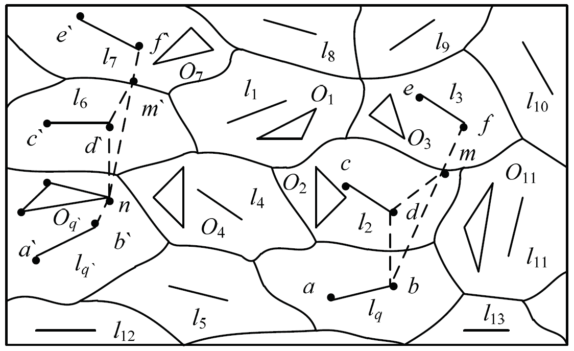
Proof. We prove the theorem by using the method of reduction. The query line segment [TeX:] $$l_{q},$$ data line segment [TeX:] $$l_{2} \text { and } l_{3}$$ are given, which as shown in Fig. 1. Supposing that the distance from the query line segment [TeX:] $$l_{q}$$ to the data line segment [TeX:] $$l_{3}$$ is closer than that to [TeX:] $$l_{2},$$ that is assuming [TeX:] $$V \operatorname{dist}\left(l_{q}, l_{3}\right)<\operatorname{Vdist}\left(l_{q}, l_{2}\right).$$ According to the line segment distance definition, the distance between [TeX:] $$l_{q} \text { and } l_{2}$$ can be expressed as [TeX:] $$V \operatorname{dist}\left(l_{q}, l_{2}\right)=\operatorname{dist}(b, d),$$ the distance between [TeX:] $$l_{q} \text { and } l_{3}$$ can be expressed as [TeX:] $$\text {Vdist}\left(l_{q}, l_{3}\right)=\operatorname{dist}(b, f)=\operatorname{dist}(b,m)+\operatorname{dist}(m, f).$$ The equation dist(m, d)=dist(m, f) will be obtained in accordance with the property of line segment Voronoi diagram. As in the Euclidean space, the triangle inequality theorem is satisfied, thus [TeX:] $$\operatorname{dist}(b, m)+\operatorname{dist}(m, d)>\operatorname{dist}(b, d), \operatorname{dist}(b, f)>\operatorname{dist}(b, d), \text { that is } \operatorname{dist}\left(l_{q}, l_{3}\right)>\operatorname{dist}\left(l_{q}, l_{2}\right).$$ The original theorem is established because of the contradiction with the hypothesis. Prove finished.
Theorem 1 is applicable to the case that there is no effective obstacle between the query line segment and the data line segment. In other words, the distance between the query line segment and its adjacent data line segment is shorter than that between other lines. For example, if is a query line segment, then [TeX:] $$\operatorname{dist}\left(l_{12}, \quad l_{5}\right)<\operatorname{dist}\left(l_{12}, l_{4}\right),$$ as shown in Fig. 1.
THEOREM 2. Given query line segment [TeX:] $$l_{q},$$ data line segment [TeX:] $$l_{i} \ and \ l_{j}.$$ From [TeX:] $$l_{q} \text { to } l_{j},$$ it needs to go through the Voronoi polygon which [TeX:] $$l_{i}$$ is in. If the effective obstacle exists between [TeX:] $$l_{q} \text { and } l_{i},$$ then [TeX:] $$Odist \left(l_{q}\right.,l_{i}) \leq O d i s t\left(l_{q}, l_{j}\right)$$.
Proof. We prove the theorem by using the method of reduction. The query line segment [TeX:] $$l_{q},$$ data line segment [TeX:] $$l_{6} \text { and } l_{7},$$ and obstacle [TeX:] $$O_{q}'$$ are given, as is shown in Fig. 1. Supposing that the obstacle distance from the query line segment [TeX:] $$l_{q}$$ to the data line segment [TeX:] $$l_{7}$$ is closer than that to [TeX:] $$l_{6},$$ that is assuming [TeX:] $$Odist \left(l_{q'}\right.\left.l_{7}\right)<\operatorname{Odist}\left(l_{q'} , l_{6}\right).$$ According to the line segment distance definition, the obstructed distance between [TeX:] $$l_{q}$$ and [TeX:] $$l_{6}$$ can be expressed as [TeX:] $$\text {Odist}\left(l_{q'} , l_{6}\right)=\operatorname{dist}(b' , n)+\operatorname{dist}\left(n, d^{\prime}\right),$$ the obstructed distance between [TeX:] $$l_{q} \text { and } l_{7}$$ can be expressed as [TeX:] $$\text {Odist}\left(l_{q'} , l_{7}\right)=\operatorname{dist}(b' , n)+\operatorname{dist}(n, f).$$ In order to prove the connection point [TeX:] $$d ' \ and \ m', \ dist (d', \left.m^{\prime}\right)=\operatorname{dist}(m', f))$$ will be obtained in accordance with the property of line segment Voronoi, therefore, [TeX:] $$\text {Odist}\left(l_{q'} , l_{7}\right)=\operatorname{dist}\left(b^{\prime}, n\right)+\operatorname{dist}\left(d^{\prime}, m^{\prime}\right)+\operatorname{dist}(m' , n).$$ According to the triangle inequality theorem, [TeX:] $$dist \ (n, \left.m^{\prime}\right)+\operatorname{dist}\left(m^{\prime}, d\right)>\operatorname{dist}\left(n, d^{\prime}\right).$$ can be obtained, thus [TeX:] $$\operatorname{dist}\left(n, b^{\prime}\right)+\operatorname{dist}\left(n, d^{\prime}\right)<\operatorname{dist}\left(n, b^{\prime}\right)+\operatorname{dist}(n, f'), \text { Odist }\left(l_{q'},\right.\left.l_{6}\right)<O d i s t\left(l_{q'} , l_{7}\right).$$ The original theorem is established because of the contradiction with the hypothesis. Prove finished.
Theorem 2 is applicable to the case that there is an effective obstacle between the query line segment and the data line segment. The effective obstacle between the two lines will certainly affect the calculation of the distance between the two lines. The existence of obstacles will increase the distance between the two lines, but compared with other data lines, the distance between the data lines adjacent to the query lines is relatively smaller. For example, suppose [TeX:] $$l_{1}$$ is a query line segment, then [TeX:] $$\text {Odist}\left(l_{1}, l_{3}\right)<\text {Odist}\left(l_{1}, l_{10}\right),$$ as is shown in Fig. 1.
According to Theorem 1 and Theorem 2, pruning rule 1, 2, 3, 4 are given as follows:
Pruning rule 1. We take the visible shortest distance from query line segment to data line segment as the radius, and generate two circles with two endpoints of [TeX:] $$l_{q}.$$ The region which they cover is marked as E. Then the k nearest neighbor of [TeX:] $$l_{q}$$ may be in the Voronoi polygon which intersects with E.
Pruning rule 2. If the data line segment in the Voronoi polygon which is adjacent to the query line segment, then it may be the k nearest neighbor of the line segment.
Pruning rule 3. If the Voronoi polygon [TeX:] $$V L\left(l_{i}\right)$$ of the data line segment and the Voronoi polygon [TeX:] $$V L\left(l_{q}\right)$$ of the query line segment have no common edge, then the data line segment [TeX:] $$l_{i}$$ is pruned.
Pruning rule 4. If the minimum number of Voronoi polygons passing from the data line segment to the query line segment exceeds k, then the data line segment will be pruned.
Based on the discussion above, the filtering algorithm is shown in Algorithm 1.
Algorithm 1
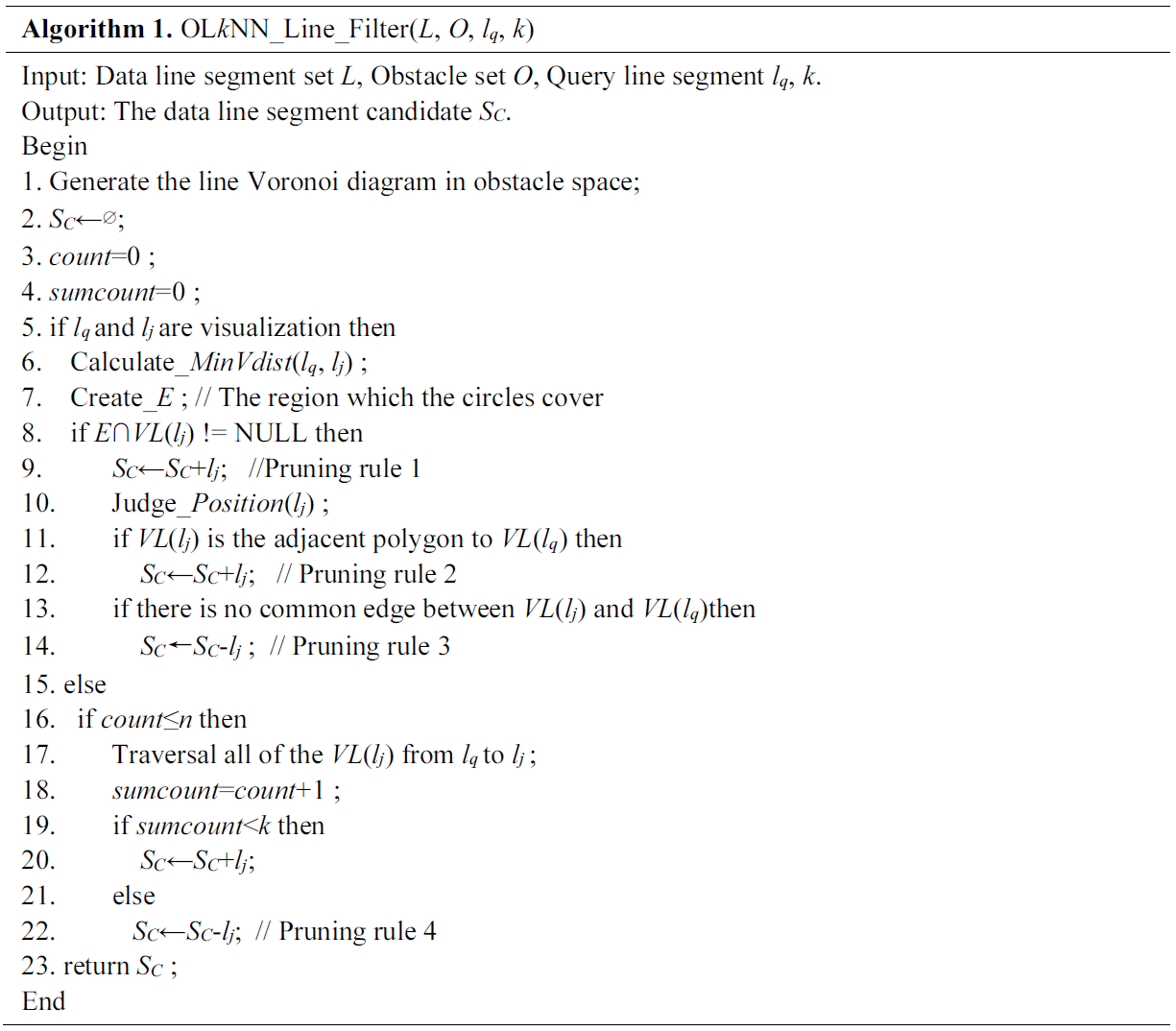
The algorithm OLkNN_Line_Filter constructs line segment Voronoi diagram through the data line segment set, and collects the obstacle which is formed by three points except from the end points of the line segment randomly in any of [TeX:] $$V L\left(l_{j}\right),$$ so that the line segment Voronoi diagram in obstacle space is formed (Line 1). The algorithm initializes data line segment candidate set [TeX:] $$S_{C},$$ and counts variables (Line 2–4). Then we can judge whether there is visible distance between query line segment [TeX:] $$l_{q}$$ and data line segment [TeX:] $$l_{j}.$$ If it exists visible distance, then we calculate it according to Pruning rule 1. We create area E to filter the data line segment (Line 5–9). If the data line segment satisfies Pruning rule 2, it will be added into data line segment candidate set SC, or it will be pruned (Line 10–12). According to Pruning rule 3, if there is no common side between [TeX:] $$V L\left(l_{q}\right) \text { and } V L\left(l_{j}\right),$$ the data line segment [TeX:] $$l_{j}$$ is pruned (Line 13–14). If there is no visible distance between query line segment [TeX:] $$l_{q}$$ and data line segment [TeX:] $$l l,$$ according to Pruning rule 4, we can have screen on data line segment by judging the number of Voronoi polygons which are covered by the route between them. The satisfied data line segment will be added into the candidate set [TeX:] $$S_{C},$$ will be formed (Line 23). We further filter the obstacle data. Given the query line segment [TeX:] $$l_{q},$$ obstacle O and data line segment l in candidate set [TeX:] $$S_{C}.$$ We connect the endpoints of the data line segment and query line segment to form a polygon P. According to the different position between obstacle and polygon P, Theorem 3 and Theorem 4 are proposed.
THEOREM 3. If obstacle [TeX:] $$O_{x}$$ has no intersection with polygon P, then obstacle [TeX:] $$O_{x}$$ is not the effective obstacle.
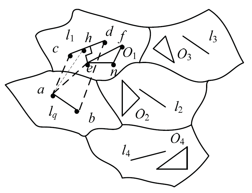
Proof. We provide query line segment [TeX:] $$l_{q}$$ and set the left and right endpoints as point a and point b respectively. Data line segment [TeX:] $$l_{1}$$ is provided, and the left and right endpoints are set as point c and point d, as is shown in Fig. 2. We connect the endpoints of data line segment and query line segment to form quadrangle abcd. The obstacle [TeX:] $$O_{2}, O_{3} \text { and } O_{4}$$ have no intersection with quadrangle abcd. When we compute the obstacle distance between query line segment [TeX:] $$l_{q}$$ and data line segment [TeX:] $$l_{1},$$ it is unnecessary to take the effect of obstacle [TeX:] $$O_{2}, O_{3} \text { and } O_{4},$$ into consideration, so obstacle [TeX:] $$O_{2}, O_{3} \text { and } O_{4}$$ are not effective obstacles. Therefore, the original theorem was established. Proof finished.
Theorem 3 is used to filter the data line segments in the previous stage. For two line segments, an auxiliary line is constructed by connecting their endpoints to form a polygon. If there is no intersection between obstacles and polygons, the distance between the two lines must not be affected. So the distance between the two lines need not be considered when the distance between the lines is calculated.
THEOREM 4. If obstacle [TeX:] $$O_{x}$$ intersected with polygon P, and it has no intersection with the shortest visual distance from query line segment to data line segment, then obstacle [TeX:] $$O_{x}$$ is not effective obstacle.
Proof. The theorem is proved by contradiction. The obstacle O1 has three endpoints: point e, point n and point f, as shown in Fig. 2. Obstacle [TeX:] $$O_{1}$$ has intersection with quadrangle abcd. Assuming that obstacle [TeX:] $$O_{1}$$ has impact on the obstacle distance from [TeX:] $$l_{q} \text { to } l_{1}$$ that is [TeX:] $$O_{1}$$ is an effective obstacle. The shortest visual distance from [TeX:] $$l_{q} \text { to } l_{1}$$ is represented as [TeX:] $$V \operatorname{dist}\left(l_{q}, l_{1}\right).$$ According to the definition of line distance, the visual distance from [TeX:] $$l_{q} \text { to } l_{1}$$ can be shown as [TeX:] $$\text {Vdist}\left(l_{q}, l_{1}\right)=\operatorname{dist}(a, c).$$ We take the effect of obstacle [TeX:] $$O_{1}$$ into consideration, the obstacle distance from [TeX:] $$l_{q} \text { to } l_{1}$$ can be represented as [TeX:] $$\text {Odist}\left(l_{q}, l_{1}\right)=\operatorname{dist}(a, e)+\operatorname{dist}(e, h).$$ From the triangle inequality theorem, we can get [TeX:] $$\text { dist }(a, e)+\operatorname{dist}(e, h)>\operatorname{dist}(a, h) . \text { So, dist }(a, h)>\operatorname{dist}(a, c),$$ that is [TeX:] $$\operatorname{dist}(a, c)<\operatorname{dist}(a, e)+\operatorname{dist}(e, h).$$ Therefore, when we compute the distance between [TeX:] $$l_{q} \text { and } l_{1},$$ it is unnecessary to take the effect of obstacle [TeX:] $$O_{1}$$ into consideration and obstacle [TeX:] $$O_{1}$$ is not the valid obstacle. It is inconsistent with the hypothesis. Therefore, the original theorem was established. Proof finished.
Theorem 4 is applicable to further judgment of effective obstacles. Assuming that two line segments are visible, the shortest visual distance between two line segments is constructed as an auxiliary line. For example, we calculate the distance between line segments [TeX:] $$l_{2} \ and \ l_{3},$$ the obstacle [TeX:] $$O_{3}$$ is an effective obstacle in Fig. 2.
Based on Theorems 3 and 4, pruning strategy 5, 6, and 7 are given as follows.
Pruning rule 5. If the obstacle is in the Voronoi polygon which candidate set SC of data line segments existed, then the obstacle may be an effective obstacle.
Pruning rule 6. If the shortest distance from query line segment to obstacle is longer than the distance to the diagonal of polygon P, then the obstacle is not an effective obstacle.
Pruning rule 7. If the shortest distance from query line segment to obstacle is shorter than the length of polygon’s diagonal line, and it also has intersection with polygon P, then the obstacle is an effective obstacle.
Based on the discussion above, the filtering algorithm is shown in Algorithm 2.
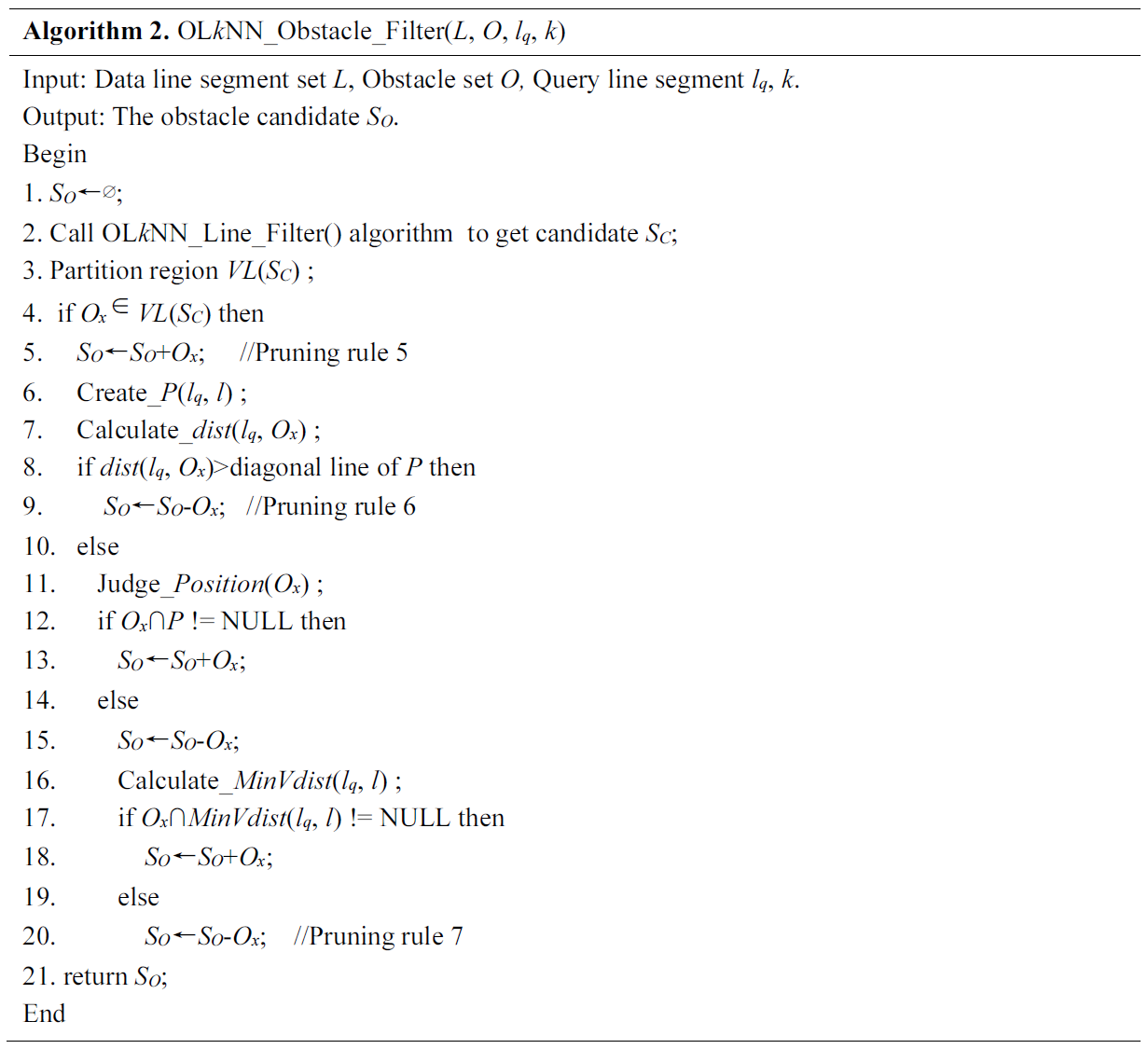
Based on the location of the data line segment in the candidate set [TeX:] $$S_{C},$$ the algorithm OLkNN_Obstacle_Filter can partition the area [TeX:] $$\left.V L\left(S_{C}\right) \text { (Line } 1-3\right).$$ Then we can make use of the Pruning rule 5 to judge whether obstacle [TeX:] $$O_{x}$$ is in area [TeX:] $$V L\left(S_{C}\right) . \text { If } O_{x}$$ has intersection with [TeX:] $$V L\left(S_{C}\right), O_{x}$$ should be added into the candidate set [TeX:] $$S_{O}(\text { Line } 4-5).$$ We form polygon P and calculate the distance from query line segment to the obstacle. According to Pruning rule 6, we judge the relation between [TeX:] $$\operatorname{dist}\left(l_{q}, O_{x}\right)$$ and length of diagonal line of P (Line 6–9). If the distance between [TeX:] $$l_{q} \text { and } O_{x}$$\ is less than the diagonal line of P, then we use Pruning rule 7 and Theorem 4 to make further judgment on obstacles, and add the satisfied obstacles into candidate set [TeX:] $$S_{O}(\operatorname{line} 10-20).$$ Finally, the filtered valid obstacle candidate set [TeX:] $$S_{O}$$ can be obtained (Line 21).
3.2 Refining Process
The refined algorithm proposed mainly has operation on the candidate set SC and SO which are produced during the filtration process. First, the shortest obstructed distance from query line segment to data line segment which is newly added to the candidate set is calculated. Then we compared the shortest obstructed distance and the more accurate result of the k nearest neighbor of line segment in obstacle environment can be obtained.
In order to represent the obstacle distance between the data line segment and the query line segment more accurately, the following theorem 5 is further proposed.
THEOREM 5. Given the data line segment l, the query line segment [TeX:] $$l_{q},$$ and the obstacle O. If there is a visual distance [TeX:] $$\text {Vdist }\left(l_{q}, l\right) \text { , then } V \text {dist}\left(l_{q}, l\right)<\text {Odist}\left(l_{q}, l\right).$$
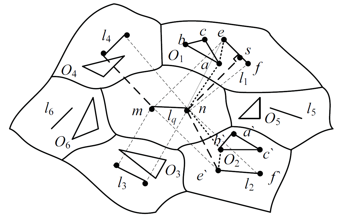
Proof. Given the set of data line segment set [TeX:] $$L=\left\{l_{1}, l_{2}, l_{3}, l_{4}, l_{5}, l_{6}\right\},$$ query line segment [TeX:] $$l_{q},$$ and the obstacle set [TeX:] $$O=\left\{O_{1}, O_{2}, O_{3}, O_{4}, O_{5}, O_{6}\right\}.$$ We create line segment Voronoi diagram as shown in Fig. 3. When there is no intersection between the obstacle and the visual distance, the visual distance can be expressed as [TeX:] $$V \operatorname{dist}\left(l_{q}, l\right),$$ such as data line segment [TeX:] $$l_{1} \ and \ l_{2}.$$ Because the location of the line segment is different, the distance representation method is different. When the two line segments are introverted, we structure the visual distance between [TeX:] $$l_{q} \text { and } l_{1},$$ that is [TeX:] $$V d i s t\left(l_{q}, l_{1}\right)=\operatorname{dist}(n, s).$$ The obstacle distance between [TeX:] $$l_{q} \text { and } l_{1}$$ is expressed as [TeX:] $$\text {Odist}\left(l_{q}, l_{1}\right)=\operatorname{dist}(n, a)+\operatorname{dist}(a, e).$$ In the Euclidean space, then [TeX:] $$\operatorname{dist}(n, a)+\operatorname{dist}(a,e)>\operatorname{dist}(n, e), \text { and } \operatorname{dist}(n, e)>\operatorname{dist}(n, s), \text { therefore } V \operatorname{dist}\left(l_{q}, l_{1}\right)<\operatorname{Odist}\left(l_{q}, l_{1}\right).$$ When the two line segments are extroverted, the visual distance between [TeX:] $$l_{q} \ and \ l_{2}$$ is constructed. As shown in Fig. 3, we can further get the visual distance [TeX:] $$\text {Vdist}\left(l_{q}, l_{2}\right)=\operatorname{dist}\left(n, e^{\prime}\right),$$ obstacle distance [TeX:] $$\text {Odist}\left(l_{q}, l_{2}\right)=\operatorname{dist}\left(n, b^{\prime}\right)+\operatorname{dist}\left(b^{\prime}, e^{\prime}\right),$$ and the inequality [TeX:] $$V d i s t\left(l_{q}, l_{2}\right)<\operatorname{Odist}\left(l_{q}, l_{2}\right)$$ can be obtained . Therefore, there is an inequality [TeX:] $$\text {Vdist}\left(l_{q}, l\right)<\text {Odist}\left(l_{q}\right.,l)$$ when there is a visual distance. Proof finished.
Theorem 5 is used to further judge the shortest distance between two lines when there are effective obstacles. For example, the data line segments [TeX:] $$l_{3}, l_{5}, l_{6}$$ and the query line segment [TeX:] $$l_{q}$$ are completely invisible in Fig. 3, so the obstacle distance should be considered. For the partial visibility between line segment [TeX:] $$l_{1}, l_{2}, l_{4}$$ and query line segment [TeX:] $$l_{q},$$ in order to get the expression of the shortest distance between two line segments, we need to use Theorem 5 to compare the obstacles distance (Odist) and visible distance (Vdist).
Based on the discussion above, further refinement algorithm for the k nearest neighbor of line segment in obstacle environment is given, shown in Algorithm 3.
Algorithm 1

First, the algorithm STA_OLkNN initializes obstacle candidate set [TeX:] $$S_{R}$$ and the obstacle distance from query line segment [TeX:] $$l_{q}$$ to data line segment l (Line 1–2). Polygon P can be formed by connecting the endpoints of the two lines, and then we can have a judgment on the visualization between query line segment and data line segment (Line 3–4). If the obstacle [TeX:] $$O_{x}$$ is intersected with the two edges of the polygon P, the data line segments and the query line segment are completely invisible, so there is no visual distance. The obstacle distance between the two lines should be expressed and further compared to get the shortest obstacle distance (Line 5–9). If there is visual distance between the data segment and the query line segment, then the visual distance can be represented. According to Theorem 5, if the visual distance is less than the obstacle distance, then the distance between the two line segments is recorded as visual distance. The algorithm further deletes the data line segments which do not meet the query requirements from the result (Line 10–14). Finally, the more accurate query result set [TeX:] $$S_{R}$$ can be obtained in the obstacle space (Line 15).
4. Experiment
In this section, the performance of the proposed algorithm is analyzed through experiments. The operating environment of the experiments is as follows: 2.0 GHZ CPU, 4 GB memory, 500 GB hard disk, Windows 7 system. The adopted data set is the road network information of the State of California [26]. In the experiment, the distribution of the target data is adjusted appropriately. Let D represent the size of the data line segment set, m represent the number of obstacles in the obstacle data set O, k represent the number of nearest neighbor of line segment in the obstacle space.
The running time of the algorithm is treated as test indicator, and each experimental result takes the average of 100 queries. Firstly, the OLkNN query algorithm (STA_OLkNN) is tested under the condition of the static obstacles. Further we test the influence of the k value, the number of obstacles m, the data set size D, and the I/O cost on the running time of the algorithm.
As the k nearest neighbor query of line segment in the obstacle environment is proposed for the first time in this paper, the existing methods of the nearest neighbor queries in obstacle space are based on points, so the proposed method cannot be directly compared with the existing research results. In order to get the comparison algorithm, this paper discussed the two nearest neighbor query algorithms which are proposed in [22] and [23]. If there is an effective obstacle between the two line segments, then we express the obstacle distance in combination of the definition of obstacle distance of line segment which is proposed in this paper. After some proper adjustments of these two algorithms, OLkNN_Basic1 and OLkNN_Basic2 are obtained.
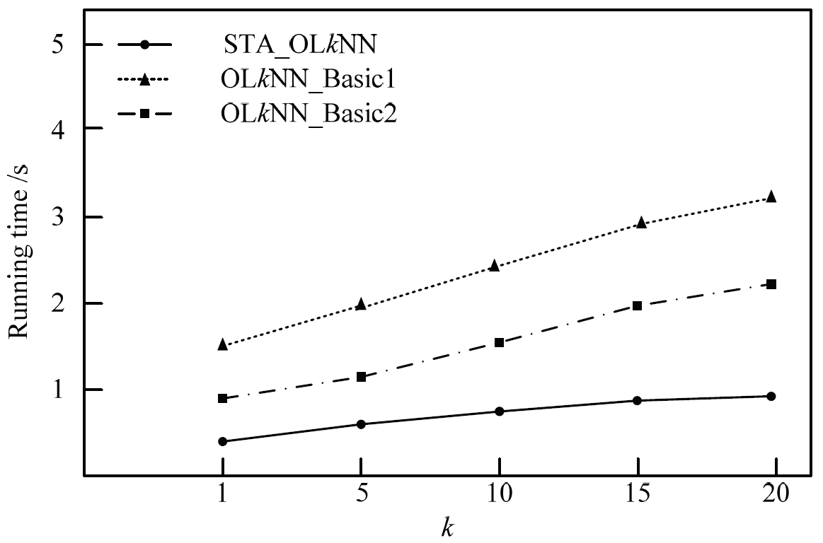
Firstly, we test the influence of k value on the running time of the algorithm. The test results are shown in Fig. 4. In this paper, the running time of CPU is increased with the k value. But the trend of the algorithm which is proposed in this paper is more smoothly. Because the two comparison algorithms need to consider the impact of all data line segments and obstacles in the query process, they will cost much CPU running time compared with the STA_OLkNN algorithm. Therefore, the proposed algorithm in this paper is superior to the two comparison algorithms in terms of running time.
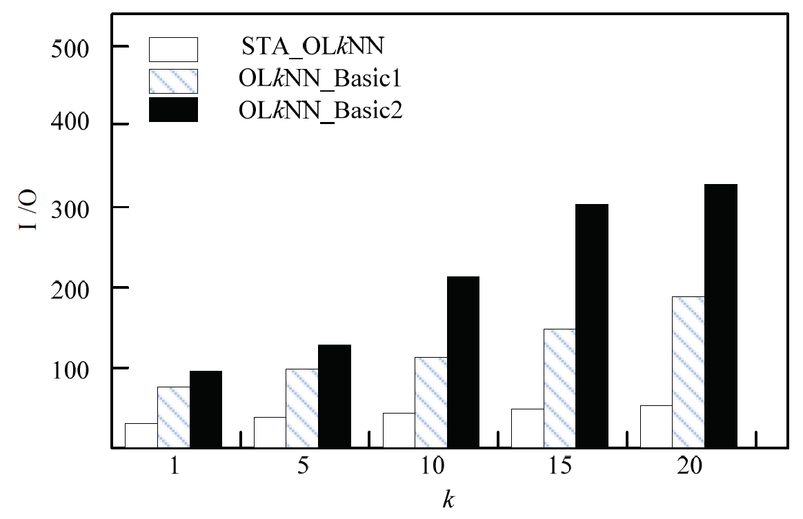
In the case of other conditions unchanged, we test the impact of k value on the cost of I/O. The test results are shown in Fig. 5. The I/O costs of STA_OLkNN algorithm and the two comparison algorithms are increased with the change of the k value. Compared with OLkNN_Basic1 and OLkNN_Basic2, in accordance with the filtering process of data line segments and obstacles, the algorithm proposed in this paper excluded a large amount of useless data and decreased data access amount, therefore, the cost of I/O is lower than that of the two comparison algorithms. It can be concluded that the STA_OLkNN algorithm proposed in this paper is better than the two comparison algorithms.
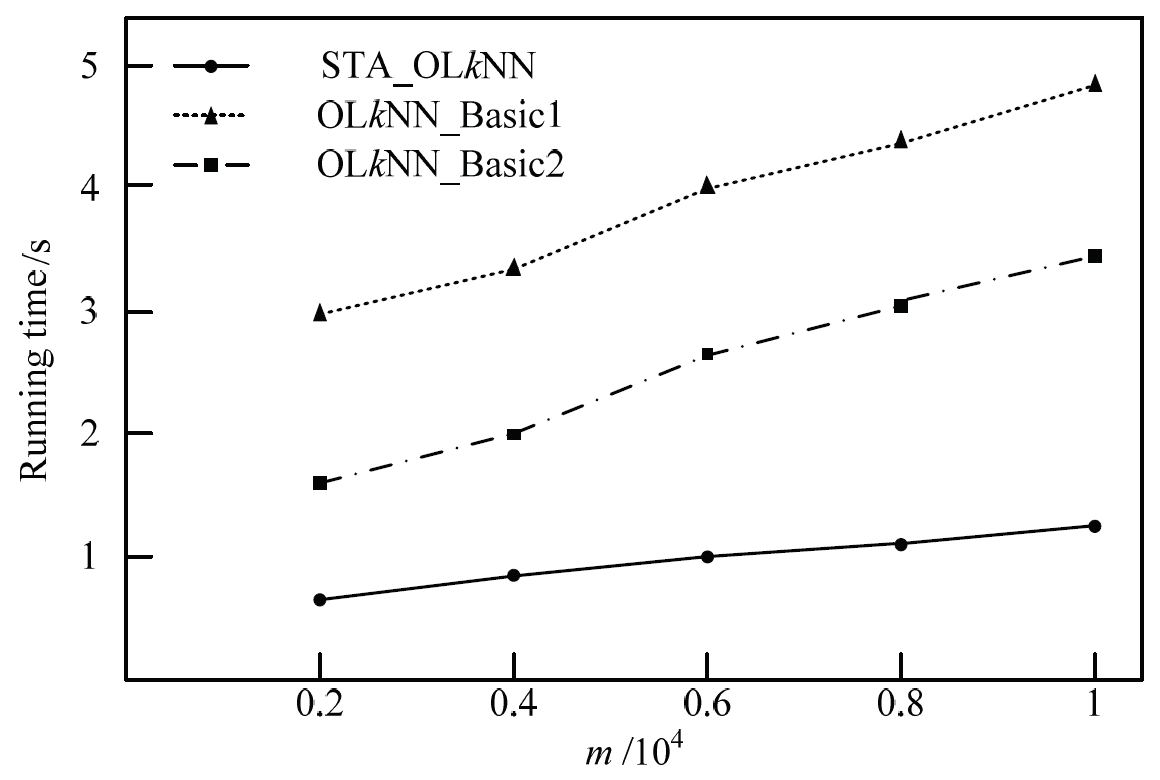
Further we test the impact of m on CPU running time. The size of the k value set is 10 and the size of data line segments set is 20000. Fig. 6 shows the change of CPU running time of these three algorithms. The experimental results show that the STA_OLkNN algorithm proposed in this paper is superior to the two comparison algorithms. Compared with OLkNN_Basic1 algorithm and OLkNN_Basic2 algorithm, the growth trend of STA_OLkNN algorithm is more smoothly. The reason for this is that it filtered obstacles in the filtering process and the number of obstacles influence on CPU running time is not too much. While the two comparison algorithms need to consider the impact of all obstacles to the query, so they will spend more running time.
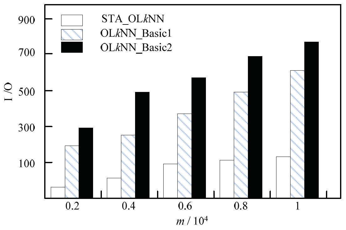
In the case of other conditions unchanged, we test the impact of m value on the cost of I/O. The experimental results in Fig. 7 show that STA_OLkNN algorithm is better than the two comparison algorithms. OLkNN_Basic1 algorithm and OLkNN_Basic2 algorithm appear a clear upward trend, the reason is that the comparison algorithms need to consider each obstacle in the process of query. With the increasing number of obstacles, the rate of the quantity of visiting data get larger.
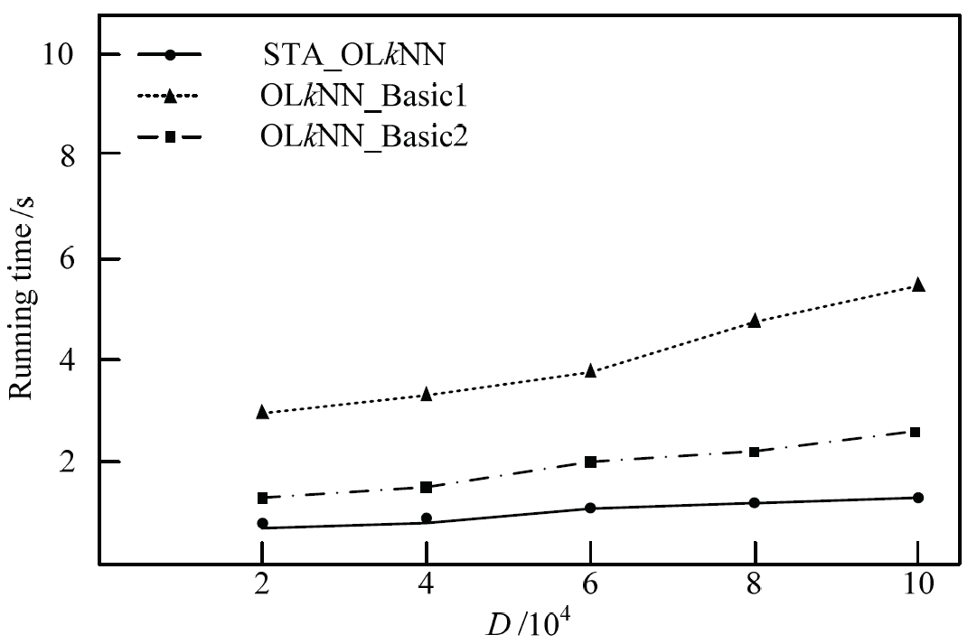
Then we test the effect of the data size D on CPU running time. We set the k value as 10 and the size of the obstacles is 2000. The experimental results are shown in Fig. 8. The STA_OLkNN algorithm can exclude a large number of non-candidate data in the filtering process, so even if the data size increases, the increasing of CPU running time of the query algorithm is not significant, the upward trend is more smoothly. For the two comparison algorithms, the CPU running time is affected greatly. Therefore, in terms of the impact of the data size on the algorithm running time, the STA_OLkNN algorithm proposed in this paper is better than the two comparison algorithms.
5. Conclusions
In this paper, the k nearest neighbor query method of line segment in obstacle space is proposed. In different situations of the line segment and the obstacle, the pruning strategies for data line segments and obstacles are proposed based on the property of the line segment Voronoi diagram. The pruning strategies can exclude a large number of non-candidate data and the efficiency of the algorithm can be improved. Then the STA_OLkNN algorithm in static obstacles space is finally obtained. Theoretical research and experimental results show that the proposed algorithm has high efficiency. The focus of future research is mainly on the nearest neighbor query of line segment in uncertain data and the skyline query for the line segment.
Acknowledgement
This paper is supported by the National Natural Science Foundation of China (Grant No. 61872105), the science and technology research project of Heilongjiang provincial education department (Grant No. 12531z004), and the Scientific Research Foundation for Returned Scholars abroad of Heilongjiang Province of China (No. LC2018030).
Biography
References
- 1 C. Efstathiades, A. Efentakis, D. Pfoser, "Efficient processing of relevant nearest-neighbor queries," ACM Transactions on Spatial Algorithms and Systems (TSAS), vol. 2, no. 3, 2016.doi:[[[10.1145/2934675]]]
- 2 S. Suri, V. V erbeek, "On the most likely voronoi diagram and nearest neighbor searching," International Journal of Computational Geometry & Applications, vol. 26, no. 3-4, pp. 151-166, 2016.doi:[[[10.1142/S0218195916600025]]]
- 3 O. F. Ertugrul, M. E. Tagluk, "A novel version of k nearest neighbor: dependent nearest neighbor," Applied Soft Computing, vol. 55, pp. 480-490. 2017. doi:[[[10.1016/j.asoc.2017.02.020]]]
- 4 C. Li, D. R. Shen, M. D. Zhu, Y. Kou, T. Z. Nie, G. Yu, "kNN query processing approach for content with location and time tags," Journal of Software, vol. 27, no. 9, pp. 2278-2289, 2016.custom:[[[-]]]
- 5 Y. Jing, L. Hu, W. S. Ku, C. Shahabi, "Authentication of k nearest neighbor query on road networks," IEEE Transactions on Knowledge and Data Engineering, vol. 26, no. 6, pp. 1494-1506, 2013.doi:[[[10.1109/TKDE.2013.174]]]
- 6 S. Dasgupta, K. Sinha, "Randomized partition trees for exact nearest neighbor search," Algorithmica, vol. 72, no. 1, pp. 237-263, 2015.custom:[[[-]]]
- 7 S. Yi, C. Shim, Y. D. Chung, "Reverse view field nearest neighbor queries," Information Sciences, vol. 402, pp. 35-49, 2017.doi:[[[10.1016/j.ins.2017.03.031]]]
- 8 A. Hidayat, S. Yang, M. A. Cheema, D. Taniar, "Reverse approximate nearest neighbor queries," IEEE Transactions on Knowledge and Data Engineering, vol. 30, no. 2, pp. 339-352, 2017.doi:[[[10.1109/TKDE.2017.2766065]]]
- 9 Z. Liu, C. Wang, J. Wang, "Aggregate nearest neighbor queries in uncertain graphs," World Wide Web, vol. 17, no. 1, pp. 161-188, 2014.doi:[[[10.1007/s11280-012-0200-6]]]
- 10 T. Hashem, L. Kulik, K. Ramamohanarao, R. Zhang, S. C. Soma, "Protecting privacy for distance and rank based group nearest neighbor queries," World Wide Web, vol. 22, no. 1, pp. 375-416, 2019.custom:[[[-]]]
- 11 A. P. Sistla, O. Wolfson, B. Xu, "Continuous nearest-neighbor queries with location uncertainty," The VLDB Journal, vol. 24, no. 1, pp. 25-50, 2015.doi:[[[10.1007/s00778-014-0361-2]]]
- 12 Y. Wang, Y. H. Dong, J. B. Qian, H. H. Chen, "Continuous nearest-neighbor query in location privacy preserving," Journal of Beijing University of Posts & Telecommunications, vol. 39, no. 5, pp. 83-88, 2016.custom:[[[-]]]
- 13 P. K. Agarwal, B. Aronov, S. Har-Peled, J. M. Phillips, K. Yi, W. Zhang, "Nearest-neighbor searching under uncertainty II," ACM Transactions on Algorithms, vol. 13, no. 1, 2016.doi:[[[10.1145/2955098]]]
- 14 Z. Liu, C. Wang, J. Wang, "Aggregate nearest neighbor queries in uncertain graphs," World Wide Web, vol. 17, no. 1, pp. 161-188, 2014.doi:[[[10.1007/s11280-012-0200-6]]]
- 15 S. Li, L. Zhang, Z. Hao, "Strong neighborhood pair query in dynamic dataset," Journal of Computer Research and Development, vol. 52, no. 3, pp. 749-759, 2015.custom:[[[-]]]
- 16 H. Zhu, J. Wang, B. Wang, X. Yang, "Location privacy preserving obstructed nearest neighbor queries," Journal of Computer Research and Development, vol. 51, no. 1, pp. 115-125, 2014.custom:[[[-]]]
- 17 X. N. Yu, Y. Gu, T. C. Zhang, G. Yu, "A method for reverse k-nearest-neighbor queries in obstructed spaces," Jisuanji Xuebao (Chinese Journal of Computers), vol. 34, no. 10, pp. 1917-1925, 2011.custom:[[[-]]]
- 18 H. Zhu, X. Yang, B. Wang, W. C. Lee, "Range-based obstructed nearest neighbor queries," in Proceedings of the 2016 International Conference on Management of Data, San Francisco, CA, 2016;pp. 2053-2068. custom:[[[-]]]
- 19 Z. Yang, Z. Hao, "Group obstacle nearest neighbor query in spatial database," Journal of Computer Research and Development, vol. 50, no. 11, pp. 2455-2462, 2013.custom:[[[-]]]
- 20 L. Zhang, L. Liu, X. Hao, S. Li, Z. Hao, "V oronoi-based group reverse k nearest neighbor query in obstructed space," Journal of Computer Research and Development, vol. 54, no. 4, pp. 861-871, 2017.custom:[[[-]]]
- 21 Z. Hao, Y. Wang, Y. He, "Line segment nearest neighbor query of spatial database," Journal of Computer Research and Development, vol. 45, no. 9, pp. 1539-1545, 2008.custom:[[[-]]]
- 22 R. Liu, Z. Hao, "Fast algorithm of nearest neighbor query for line segments of spatial database," Journal of Computer Research and Development, vol. 48, no. 12, pp. 2379-2384, 2011.custom:[[[-]]]
- 23 Z. Yi, Z. Yang, "Research on line segment kNN query in spatial database," Computer Engineering and Applications, vol. 51, no. 18, pp. 131-134, 2015.custom:[[[-]]]
- 24 Y. Gu, H. Zhang, Z. Wang, G. Yu, "Efficient moving k nearest neighbor queries over line segment objects," World Wide Web, vol. 19, no. 4, pp. 653-677, 2016.doi:[[[10.1007/s11280-015-0351-3]]]
- 25 M. Held, "VRONI: an engineering approach to the reliable and efficient computation of V oronoi diagrams of points and line segments," Computational Geometry, vol. 18, no. 2, pp. 95-123, 2001.custom:[[[-]]]
- 26 KONECT, 2016;, http://konect.uni-koblenz.de/networks/roadNet-CA
