Xuegang Luo , Hongrui Yu , Junrui Lv and Juan Wang
Water Quality Prediction Model Based on Tucker Decomposition and GRU-Attention Mechanism
Abstract: The issue of water pollution critically affects all living beings. The implementation of a smart water quality monitoring system, based on the Internet of Things, enables advancements in efficiency, security, and cost-effectiveness while providing real-time capabilities. Current water quality prediction models often fail to fully utilize data characteristics shared by water quality indicators, resulting in poor predictive accuracy. This study introduces a novel water quality prediction model named TGMHSA, which utilizes tensor decomposition combined with a gated neural network and a multi-head self-attention mechanism. The aim is to tackle the difficulty of forecasting water quality indicators using time series data while minimizing the risk of plagiarism. The proposed model utilizes standard delay embedding transformation (SDET) to convert the time series data into tensor data, extracting data characteristics by Tucker tensor decomposition, and then combines a multi-head self-attention mechanism to discover potential relationships among data characteristics of multiple water quality indicators. Finally, the utilization of the GRU model enables accurate prediction of multi-index water quality. In order to compare its performance, we consider four indices: root mean square error (RMSE), mean absolute error (MAE), mean absolute percentage error (MAPE), and coefficient of determination represented 2as R . The outcomes demonstrate that this model outperforms traditional methods for predicting water quality in terms of accuracy and resilience, thereby establishing a scientific foundation for effective water quality prediction and environmental monitoring management.
Keywords: Encoder-Decoder Network , Tensor Decomposition , Water Quality Prediction
1. Introduction
With the rapid development of the social economy, population growth, and urbanization, the water demand is increasing. As people's living standards and health awareness improve, they require higher drinking water quality standards. Water pollution control and restoration are becoming increasingly important, posing new challenges to water quality managers in terms of pollution control and climate change's impact on available water resources. Hence, the creation of a suitable water quality prediction model that utilizes past data from water quality monitoring to anticipate future variations in both water quality and regional indicators will greatly assist personnel tasked with overseeing and controlling aquatic environments. This timely management and forecasting will play a vital role in protecting our invaluable water resources.
The prediction of water quality indicators is a typical time series problem that can be addressed through three main types of mathematical model-based methods: time series regression analysis, machine learning, and artificial neural network composite models. Time series regression analysis builds a mathematical model based on the inertia of the data. Qin and Fu [1] proposed an autoregressive model for monitoring water quality anomalies, whose predictive efficacy is contingent upon the historical data and parameters of the regression model. Khan et al. [2] proposed the use of the principal component regression method and gradient lifting classifier for water quality prediction and classification. Hajirahimi and Khashei [3] employed an optimal bi-component series-parallel structure for the prediction of data. This model presents the benefit of enhanced accuracy in short-term indicators, posing a challenge in meeting the prediction needs for water quality management. Additionally, it is necessary to ensure stability or pre-process the data appropriately to fulfill the prerequisites of this model. The traditional approach to machine learning involves utilizing a machine simulator for parameter optimization, with ongoing refinement throughout the learning process. For instance, one method that combines support vector regression and genetic algorithm is used to predict water quality indicators [4]. Maddah [5] utilized regression-based analytical models for dissolved oxygen in wastewater. The application of the Naive Bayesian method [6] enables the prediction of water quality index, reducing reliance on raw data and minimizing the influence of noisy data on predictive outcomes. This approach is well-suited for water quality prediction due to its capability to extract features from complex machine algorithms; nevertheless, it lacks interpretability.
Most models are constructed by selecting a water distribution index to forecast future changes in water quality. Recently, numerous studies have focused on the composite model of artificial neural networks, which leverages the unique strengths of multiple networks to create a robust prediction model. For instance, a research conducted by Zhou et al. [7] introduced a model called CNN-LSTM to forecast the concentration of dissolved oxygen (DO) in water quality. This approach involves employing convolutional neural network (CNN) layers to extract features from input data and integrating them with long short-term memory (LSTM) neural network, which falls under the category of recurrent neural network (RNN). The reliability and authenticity of the data play a crucial role in determining the accuracy of the model's predictions. In order to improve the forecasting performance of the CNN-LSTM model, Mei et al. [8] introduced a hybrid approach called CNN-GRU-Attention, which effectively predicts drinking water source quality by taking into account potential pollution from industrial and agricultural activities. This method has optimized the predictive effect of traditional LSTM to some extent. This model employs CNN to extract data characteristics in either the frequency or time domain, followed by incorporating the LSTM model for prediction. However, it only predicts one of the water quality indicators and disregards the impact of interactions among these indicators on predicting them. According to Babu and Reddy [9], a prediction model named ARIMA-ANN is proposed, which enhances forecasting accuracy by integrating nonlinear artificial neural networks with linear auto-regressive integrated moving average.
To investigate the correlation between indexes, a composite neural network-based multivariate water quality parameter prediction (MWQPP) model was proposed by Wang et al. [10]. The recurrent gate unit-based prediction model effectively addresses the issue of excessive LSTM training parameters and takes into account the impact of various water quality indices, resulting in improved predictions for multiple indices. However, it lacks a feature extraction operation, resulting in training on a large amount of noise data and still exhibiting deficiencies in prediction accuracy. A hybrid water quality prediction model, which integrates artificial neural networks with wavelet transform and LSTM, was proposed in [11]. Zhou et al. [12] introduced a water quality prediction method based on an improved grey correlation analysis (IGRA) algorithm and LSTM. In addition, an integrated deep neural network combining LSTM and encoder-decoder neural network was introduced in [13,14]. Prasad et al. [15] introduced machine learning (ML) algorithms to compare AutoML with an expert-designed architecture for water quality prediction, aiming to evaluate the Water Quality Index that provides a comprehensive assessment of water quality. Deep learning approaches were proposed by [16-18] to utilize automatic and accurate prediction of key water quality parameters.
In recent years, attention-based neural networks [16,17] have been extensively utilized in the domain of natural language processing. By assigning varying weights to the hidden layer elements of the neural network, this mechanism effectively accentuates the impact of the key feature prediction model. Attention mechanisms have also been effectively utilized in certain time series forecasting investigations.
Due to the periodic characteristics of network architectures like RNN and LSTM, there is a tendency for the training process to encounter issues such as gradient disappearance or amplification. To overcome this limitation, researchers have devised a prediction model [18] that utilizes the self-attention mechanism of Transformers, which has shown impressive performance in forecasting tasks. The accurate prediction and evaluation of water quality using traditional methods pose challenges due to the influence of various environmental factors on monitoring indicators and the intricate correlation among multiple sensors. Therefore, there is still a gap in the literature survey in this study. The literature survey highlights the efficacy of soft computing approaches in predicting multi-index water quality. Furthermore, numerous investigators/researchers have employed soft computing approaches to predict critical indicators of water quality monitoring, such as DO and nitrate nitrogen (NN). However, the optimal architectural models for these predictions remain a subject of debate. Additionally, the exploration of tensor decomposition to exploit spatial relationships among multiple indicators' water quality time series data remains unexplored in current literature.
Based on this premise, we have developed a TGMHSA model that utilizes Internet of Things sensor data to predict water quality indicators. This addresses the limitation of the LSTM model in effectively highlighting important features. Initially, we integrate the data with the standard delayed embedded transformation (SDET) in a high-dimensional space. Then, we employ tensor decomposition feature data fusion gated recurrent unit (GRU) and multiple self-attention mechanisms to construct our model. To improve its ability to generalize, Tucker tensor decomposition is applied to minimize the impact of noisy data on prediction outcomes. Ultimately, experimental results demonstrate that our prediction model combining tensor decomposition and GRU achieves considerable accuracy and an improved fitting effect, thereby showcasing its robustness and precision.
The main goals of this study are to improve the precision of forecasting water quality in a watershed by implementing adaptive learning techniques on multivariate time series data and investigating the spatial correlations among various indicators. The research significance of our proposed model lies in its ability to predict key water quality parameters in sewage treatment processes based on the TGMHSA model. This prediction has significant implications for online monitoring, as it aligns more closely with the dynamic characteristics of sewage treatment systems and facilitates abnormal alarm systems.
2. Tensor Decomposition and GRU-Attention
2.1 Delayed Transformation
The precision and reliability of data are the primary determinants of model prediction performance. In low-dimensional data, features may be obscured by objects that are difficult to uncover. Moreover, municipal waste and chemical emissions from factories can impair the sensors utilized in experiments, resulting in biased data collection or inevitable noise. Therefore, the incorporation of feature selection into model building, extraction, and utilization of hidden features can significantly enhance the accuracy of prediction models.
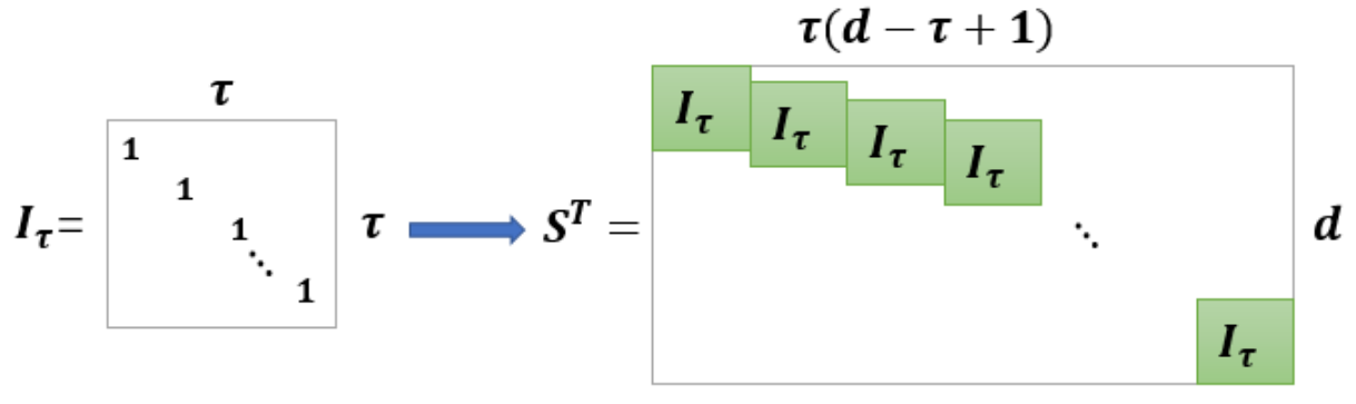
The SDET is a transformation method that expands time series data into higher-order tensors. This technique enables the conversion of small sample data into multidimensional data with larger volumes and superior characteristics, such as low-rank structured features. Set [TeX:] $$v=\left(v_1, v_1, \cdots, v_{\mathrm{n}}\right)^{\mathrm{T}} \in \mathbb{R}^{n \times d}$$ collect index values matrix for water quality sensors such as water temperature, pH (acidity-alkalinity), conductivity, DO, NN, total nitrogen content (TN), total phosphorus content (TP) from [TeX:] $$i_1 \text { to } i_{\mathrm{n}}, V_{\mathrm{j}} \in \mathbb{R}^d$$ is the data vector of d collected indices at j-time. Using block Hankel matrix S, the index data is expanded to a higher-order tensor. The matrix structure is shown in Fig. 1, and [TeX:] $$I_\tau \in \mathbb{R}^{\tau \times \tau}$$ is a unit diagonal matrix, τ is the diagonal matrix length parameter, the data 𝑉 is multiplied by the matrix S along the time direction, then the matrix is folded into a time dimension and collapsed into a tensor [TeX:] $$\mathcal{V} \in \mathbb{R}^{n \times k \times t} .$$
2.2 Tucker Tensor Decomposition
Discovering effective features in low dimensions directly is challenging. However, the SDET operation can effectively extend to high dimensions and mine features that are not observable in low dimensions. Therefore, the proposed model employs the SDET algorithm to expand the data, followed by folding it into a high-dimensional structure and applying the Tucker tensor decomposition algorithm to extract relevant features for noise reduction. The flow of data transformation and tensor decomposition is illustrated in Fig. 2. Tucker tensor decomposition breaks down the original data into a core tensor and three-factor matrices, which replace the original data. The low-rank core tensor preserves the characteristics of the original data while also possessing advantages such as small size and strong anti-interference capability.
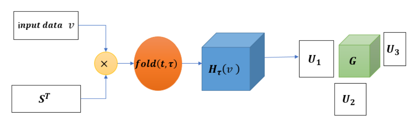
[TeX:] $$v \in \mathrm{R}^{n \times d}$$ in Fig. 2 is input data, [TeX:] $$S^{\mathrm{T}} \in \mathbb{R}^{d \times \tau(d-\tau+1)}$$ is the replication matrix, [TeX:] $$\mathrm{H}_\tau(X) \in \mathbb{R}^{J_1 \times J_2 \times J_3}$$ is the high-dimensional tensor generated by SDET, [TeX:] $$\mathcal{G} \in \mathrm{R}^{r_1 \times r_2 \times r_3}$$ is the core tensor, [TeX:] $$\left\{U^{(m)} \in \mathbb{R}^{I_m \times r_m}\right\}_{m=1}^3$$ is three-factor matrixes. The Tucker tensor decomposition steps are given in Algorithm 1.
2.3 GRU Model
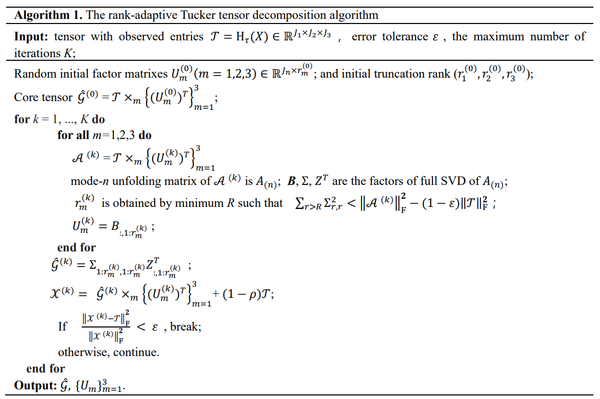
The LSTM model, known as long short-term memory, is a specialized form of RNN. It is important to note that LSTM has a complex architecture and requires lengthy training processes. This complexity leads to higher costs for network training and an increased risk of overfitting. Consequently, these factors may hinder the effectiveness of LSTM in accurately predicting water quality monitoring scenarios. To tackle the limitations of standard RNNs, a simplified version of LSTM called GRU was introduced by resetting and updating gates to address problems like slow training speed and overfitting during LSTM training. Fig. 3 depicts the structure of a single neuron in GRU, which enables it to selectively retain valuable information while discarding unnecessary data. The gating unit effectively manages the accumulation of hidden states over time, thereby resolving issues related to gradient vanishing and exploding while preserving the original functionality of LSTM and enhancing training efficiency.
In Fig. 3, [TeX:] $$X_{i-1}$$ represents input data, [TeX:] $$R_i$$ means reset gate, [TeX:] $$Z_i$$ means update gate, [TeX:] $$H_{i-1}$$ denotes the hidden state of the previous moment, [TeX:] $$\widetilde{H}_{\mathrm{i}}$$ denotes the candidate's hidden state. To begin with, activate the reset gate in order to store relevant information from the previous time step into fresh memory content. Following that, conduct element-wise multiplication between the input vector and hidden state using their respective weights. Then, perform element-wise multiplication between the reset gate and the previously multiplied hidden state. After combining these steps, apply a nonlinear activation function to generate the subsequent sequence. By employing this structure, GRU effectively captures temporal dependencies in historical data while minimizing duplication rates when being assessed for similarity. The formulas for calculating these parameters are provided.
(1)
[TeX:] $$R_{\mathrm{i}}=\sigma\left(X_{\mathrm{i}} W_{\mathrm{xr}}+H_{\mathrm{i}-1} W_{\mathrm{hr}}+b_{\mathrm{r}}\right)$$
(2)
[TeX:] $$Z_{\mathrm{i}}=\sigma\left(X_{\mathrm{i}} W_{\mathrm{xz}}+H_{\mathrm{i}-1} W_{\mathrm{hz}}+b_{\mathrm{z}}\right)$$
(3)
[TeX:] $$\widetilde{H}_{\mathrm{i}}=\tanh \left(X_{\mathrm{i}} W_{\mathrm{xh}}+\left(R_{\mathrm{t}} \odot H_{\mathrm{i}-1}\right) W_{\mathrm{hh}}+b_{\mathrm{h}}\right)$$
(4)
[TeX:] $$H_{\mathrm{i}}=Z_{\mathrm{i}} \odot H_{\mathrm{i}-1}+\left(1-Z_{\mathrm{i}}\right) \odot \widetilde{H}_{\mathrm{i}} .$$2.4 Attention Mechanism
It has been reported that LSTM and other models do not exploit the association between index values, leading to suboptimal accuracy in multi-index prediction. Our analysis reveals a strong correlation among various physical attributes in the natural environment, such as humidity, temperature, and conductivity. However, many existing methods heavily rely on historical data of these indices while neglecting the potential benefits of considering their correlated attributes. Attention mechanism, introduced by the pioneering Transformer architecture for natural language processing tasks, exclusively relies on attention mechanisms to process input sequences.
This technique has made a significant impact on deep learning and has inspired further advancements in this field. The attention mechanism, originally designed to enhance encoder-decoder RNNs for tasks like machine translation, forms the basis of the Transformer model.
It consists of a pair of sequential actions.
Step 1: Calculate the attention distribution by finding the correlation between each pair of input vectors, which is represented as α:
where [TeX:] $$S\left(x_i, q\right)$$ denotes a function for the attention scoring, which can be obtained using different models, such as the additive model, dot product model, and bilinear model.
Step 2: Once we have the attention distribution, we can weigh and average the input vectors to get a final representation of the entire sequence.
3. The Proposed TGMHSA Model
3.1 Multiple-Headed Self-Attention Mechanism
Multi-Head Self-Attention (MHSA) was initially introduced by Child et al. [16]. MHSA involves linearly mapping trainable Query Q, Key K, and Value V parameters for n iterations (where n represents the number of heads) to obtain multiple sets of distinct subspace representations. By leveraging the matching between Q and K, we can determine the influence of other features on current features through normalization and multiplication with V, thereby obtaining specific impact magnitudes. Through utilizing multiple embeddings, MHSA effectively captures crucial local information and generates a training set that encapsulates its characteristic influences. This training set exhibits heightened feature correlation levels and better reflects associations among water quality indicators. Consequently, to capture the global inter-correlation of monitoring indicators, we employ a multi-head self-attention mechanism to aggregate the information to exploit the relationships among multiple features.
Firstly, MHSA works through the embedding layer mapping the feature data [TeX:] $$\left\{a_i^n\right\}_{n=1}^N$$ obtained by Tucker tensor decomposition from raw data at the moment [TeX:] $$i,\left\{\bar{X}_i^n\right\}_{n=1}^N$$ to a higher dimension.
The node's feature vectors are transformed using three distinct matrices, namely [TeX:] $$\mathrm{W}^{\mathrm{Q}}, \mathrm{~W}^{\mathrm{K}} \text {, and } \mathrm{W}^{\mathrm{V}} \text {. }$$ This transformation yields three resulting vectors: Query, Key, and Value (as explained in the preliminaries). The parameters [TeX:] $$\mathrm{W}^{\mathrm{Q}}, \mathrm{~W}^{\mathrm{K}} \text {, and } \mathrm{W}^{\mathrm{V}} \text {. }$$ are continuously optimized and updated during model training. By taking the inner product of each node's Query vector with the Key vector of all nodes, we can utilize the softmax function to compress the resulting vector within a range of 0 to 1.
(7)
[TeX:] $$\text { Head }_{\mathrm{i}}=\operatorname{Attention}\left(\mathrm{W}_{\mathrm{i}}^{\mathrm{Q}}, \mathrm{~W}_{\mathrm{i}}^{\mathrm{K}}, \mathrm{~W}_{\mathrm{i}}^{\mathrm{V}}\right)=\operatorname{softmax}\left(\frac{Q K}{\sqrt{d_k}}\right) V,$$where [TeX:] $$\mathrm{d}_{\mathrm{k}}$$ is the dimension of the vector, [TeX:] $$Q=a_i \mathrm{~W}_{\mathrm{i}}^{\mathrm{Q}}, K=a_i \mathrm{~W}_{\mathrm{i}}^{\mathrm{K}} \text { and } V=a_i \mathrm{~W}_{\mathrm{i}}^{\mathrm{V}} .$$ By [TeX:] $$\text { Head }_{\mathrm{i}}$$ calculation, the overall attention score of this particular node can be acquired by considering its relationship with all other nodes, and subsequently combining them through an additional linear mapping to obtain the ultimate outcome.
(8)
[TeX:] $$\text { MutilHead }=\text { Concat }\left(\text { head }_1, \cdots, \text { head }_n\right) W^0$$Concat splices multiple heads and multiplies the result by a matrix [TeX:] $$W^0$$ to produce a data structure where each feature contains the influence of other features. The matrix [TeX:] $$W^0$$ is responsible for transforming the outcome of the stitching process. Output [TeX:] $$\left\{y_i^n\right\}_{n=1}^N$$ are obtained by the MutiHead function.
3.2 Overall Architecture of TGMHSA
To enhance the prediction of water quality using multiple indices, we propose a hybrid model called TGMHSA, which integrates Tensor decomposition, GRU, and MHSA architecture. After preprocessing the data, we designed a composite neural network comprising MHSA, GRU, and fully connected (FC) layers. To enhance the efficiency and stability of gradient descent in our model, we have integrated both mini-batch gradient descent (MBGD) and ADAptive Moment estimation (ADAM) optimization algorithms.
The TGMHSA algorithm partitions the dataset into multiple mini-batches for sequential training, allowing weight and bias updates after each batch. This enables frequent adjustments within a single epoch, resulting in faster convergence during gradient descent. Although various factors can influence the speed of gradient descent during training making it somewhat stochastic in nature; however machine-based gradient descent is more stable and less prone to large oscillations. In this model, we have chosen to configure the mini-batch size as 64.
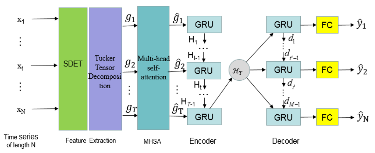
In terms of its model structure, the TGMHSA model comprises six distinct layers in its model structure: an input layer, a Tucker-feature layer employing tensor decomposition techniques, a multi-head self-attention layer for capturing interdependencies among features, a multi-module GRU layer for sequential modeling, a parallel FC layer to enhance stability and simulate complex relationships among water quality indices, and finally an output layer responsible for generating predictions of water quality index values at specific target times. To enhance the precision of prediction, this study proposes a novel encoder-decoder neural network architecture, as depicted in Fig. 4.
4. Experiments
To validate the TGMHA model, eight commonly used water quality monitoring indicators were selected as prediction targets: pH value, DO, NN, TN, chloramines, conductivity, organic carbon (OC) and trihalomethanes. We have chosen several benchmark models, such as CNN-LSTM, ARIMA-ANN, and CNN-GRU-Attention, to compare with our proposed method in terms of the predictive performance of the Water Quality Index.
4.1 Experimental Environment
The water quality index data selected from https://github.com/Abdurrahmans/ provides water quality metrics for 3,276 distinct bodies of water. The dataset is divided into three distinct subsets, specifically the training, testing, and prediction set, with a distribution ratio of 60:20:20. The Microsoft Windows 10 operating system utilizes this model, along with three other artificial neural network models, within the TensorFlow framework using the Python language.
4.2 Data Preprocessing and Model Evaluation Indexes
To enhance prediction accuracy, it is necessary to normalize each feature in the training set due to significant differences in their data. For this experiment, min-max standardization was utilized for data normalization. The formula is
Data normalization maps the original data to [0,1] to eliminate errors caused by differences in feature quantities. The model evaluation criteria include root mean square error (RMSE), mean absolute percentage error (MAPE), mean absolute error (MAE), coefficient of determination (R2).
4.3 Model Training and Evaluation
The pre-processed dataset is fed into the model for training, with the ADAM optimizer selected as the optimization function during training. Instead of using all samples at once, one mini-batch is chosen and gradient descent is employed to update model parameters. This approach addresses the issue of random small batch sampling and proves more suitable for smaller sample sizes after tensor decomposition than the traditional ADAM optimizer. In this study, the ADAM optimizer was utilized with its default parameters for training purposes.
The TGMHA model is characterized by the following parameters: it utilizes five autoregressive terms without any differencing applied and incorporates an additional three moving average terms. The dimensions of both the training set features and labels are (8, 900) and (8, 40), respectively. Similarly, the test set features and labels have dimensions of (8, 900) and (8, 40). During core tensor training, a total of 50 iterations are performed until reaching a convergence criterion of 0.001. The rank of the core tensor is specified as (5,5). Moreover, the self-attention mechanism consists of four heads with GRU hidden units optimized at a value of 256 for optimal performance. A learning rate equal to .01 is utilized while maintaining a batch size equal to one throughout the duration encompassing 20 thousand iterations.
4.4 Comparative Analysis
To assess the precision of the model, we conduct a comparative analysis between the empirical findings and forecasts generated by three distinct predictive models: ARIMA-ANN, CNN-LSTM, and CNN-GRU-Attention. These models utilize similar data processing techniques and refined training methodologies.
Table 1.
| Water Quality Index | Prediction model | MAE | RMSE | MAPE | R2 |
|---|---|---|---|---|---|
| pH | Our proposed | 0.178 | 0.189 | 0.127 | 0.894 |
| ARIMA-ANN | 0.358 | 0.358 | 0.247 | 0.689 | |
| CNN-LSTM | 0.247 | 0.289 | 0.198 | 0.786 | |
| CNN-GRU-Attention | 0.214 | 0.234 | 0.177 | 0.824 | |
| Conductivity | Our proposed | 0.258 | 0.178 | 0.147 | 0.769 |
| ARIMA-ANN | 0.356 | 0.252 | 0.273 | 0.721 | |
| CNN-LSTM | 0.319 | 0.253 | 0.180 | 0.756 | |
| CNN-GRU-Attention | 0.289 | 0.219 | 0.169 | 0.761 | |
| Chloramines | Our proposed | 0.478 | 0.547 | 0.478 | 0.789 |
| ARIMA-ANN | 0.566 | 0.658 | 0.581 | 0.748 | |
| CNN-LSTM | 0.519 | 0.589 | 0.529 | 0.769 | |
| CNN-GRU-Attention | 0.482 | 0.572 | 0.493 | 0.781 | |
| Organic-carbon | Our proposed | 0.278 | 0.204 | 0.256 | 0.714 |
| ARIMA-ANN | 0.328 | 0.321 | 0.283 | 0.679 | |
| CNN-LSTM | 0.295 | 0.260 | 0.260 | 0.701 | |
| CNN-GRU-Attention | 0.286 | 0.241 | 0.258 | 0.711 |
Table 1 presents the error assessment outcomes of the four models for pH, conductivity, chloramines, and OC four water quality indicators. All TGMHSA indexes exhibit superior performance compared to ARIMA-ANN. CNN-LSTM, on the other hand, displays a 47.2% increase in RMSE and a 48.5% increase in MAPE with MAE of 50.2%. Additionally, it shows a decrease of 29.7% in the coefficient of determination. Compared to CNN-LSTM, the RMSE exhibits a 34.6% increase, the average absolute percentage error shows a 35.8% rise, the average absolute error demonstrates a 27.9% growth, and the coefficient of determination presents an improvement of 13.7%. In comparison with CNN-GRU-Attention, the RMSE displays an increase of 19.2%, the average absolute percentage error indicates a rise of 28.2%, the average absolute error manifests an enhancement of 16.8%, and the coefficient of determination reveals an improvement by 8.4%. Specifically, SDET and Tucker tensor decomposition techniques effectively eliminate potential noise from water quality time series, while GRU and MHSA mechanisms enable the investigation of nonlinear characteristics in complex aquatic environments.
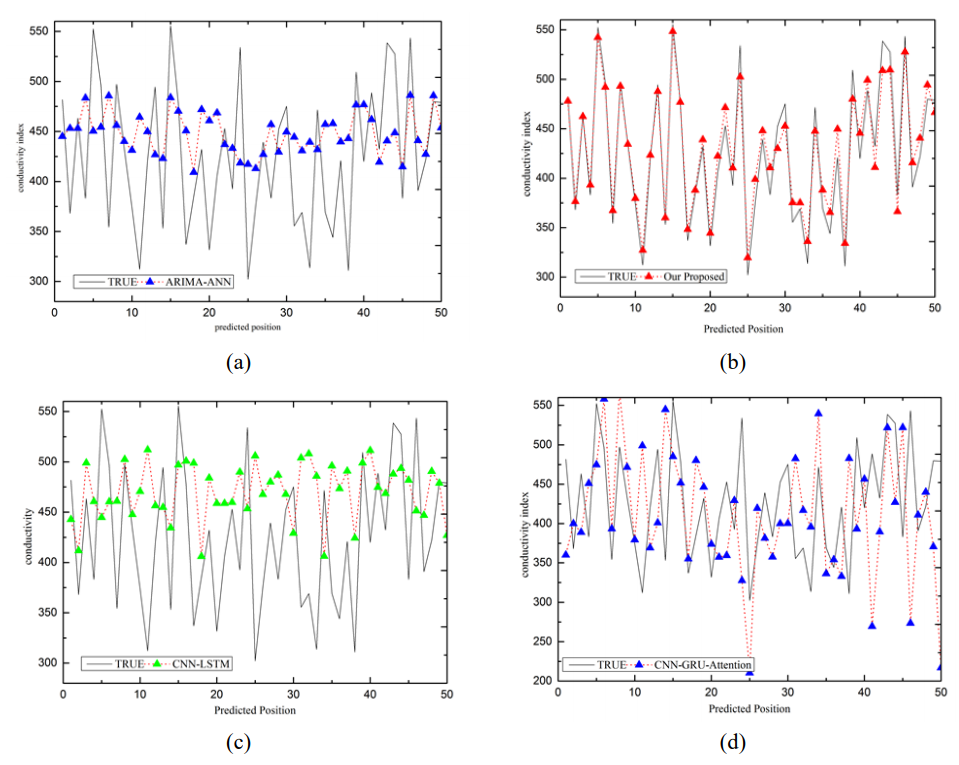
To assess the stability and robustness of the model, conductivity index has been selected for comparison. Fig. 5 depicts a comparative analysis between the predicted true values, ARIMA-ANN, CNN-LSTM, and CNN-GRU-Attention models and our proposed model.
Upon comparison between the ARIMA-ANN model and both CNN-LSTM and CNN-GRU-Attention models, we observe that while our proposed model and CNN-GRU-Attention are effective predictors, The estimated value aligns with the actual trend and deviates only slightly in specific values.
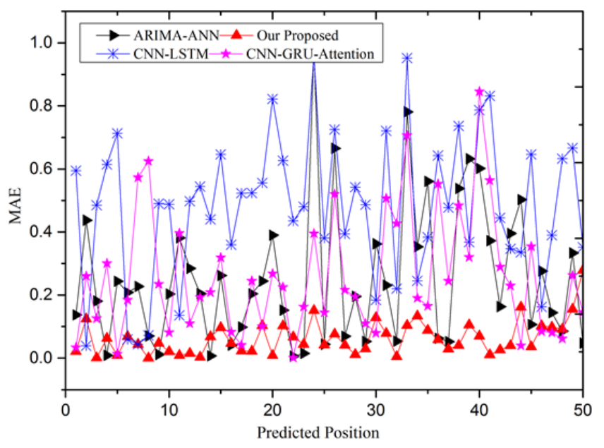
Fig. 6 demonstrates the effectiveness of our proposed model in predicting pH values by showcasing a lower error rate in MAE loss. The predicted numbers align well with the actual trend, exhibiting minimal deviation from the specific value. Our model achieves an impressive reduction in MAE to approximately 0.12 and maintains stability with further decrease to about 0.03. Based on prediction evaluation or error statistics, the performance of the TGMHSA model is more balanced, superior, and applicable to predicting multivariate water quality indicators. Furthermore, we conducted an objective comparison of experimental results with previous studies and found that our proposed multi-head mechanism model can indeed achieve outstanding performance. MHSA mechanism has also played an important role in simultaneously capturing the global and local multi-sensors correlations.
5. Conclusion
A novel approach for predicting water quality is proposed to improve the accuracy of predicting correlations and time series in water quality. The study concludes that (1) a novel approach combining tensor decomposition-GRU with multi-head self-attention mechanism fusion is suggested to enhance the accuracy of predicting correlations and time series. By incorporating GRU-based algorithms, the model's predictive capability is significantly improved, leading to a notable enhancement in the temporal correlation of water quality data. (2) Thirteen traditional and new evaluation indicators are utilized to assess the performance and accuracy of the optimized model. In summary, this research successfully employs an ADAM-optimized TGMHSA model for accurately forecasting multivariate indexes related to water quality. The outstanding performance of the TGMHSA model demonstrates its high computational efficiency for conserving water resources. Future work aims at enhancing model convergence and stability when dealing with diverse training data sources and unpredictable data conditions.
Biography
Xuegang Luo
https://orcid.org/0000-0001-8240-5199
He received B.S. degree in School of Computer Science and Engineering from Huazhong Agricultural University in 2005, and received the M.S. degree from University of Electronic Science and Technology, China, in 2008, and Ph.D. degrees from Chengdu University of Technology, China, in 2015. His current research interests include logistics optimization and machine learning.
Biography
Biography
Junrui Lv
https://orcid.org/0000-0002-6796-3819
She received B.S. degrees in School of Computer Science and Engineering from Central South University, China, in 2005 and M.S. degrees in Software College from University of Electronic Science and Technology, China, in 2009. Her current research interests include logistics optimization and image processing.
Biography
Juan Wang
https://orcid.org/0000-0003-2635-8804
She received a B.S. degree in School of Computer Science from China West Normal University, in 2003, and received the M.S. degree from China West Normal University, in 2006, and Ph.D. degree from Chengdu University of Technology, China, in 2015. She is currently an associate professor with the School of Computer Science, in China West Normal University. Her research interests include medical image processing and image fusion and image classification.
References
- 1 W. Qin and Y . Fu, "Research on water quality anomaly detection based on vector autoregression model," Journal of Safety and Environment, vol. 18, no. 4, pp. 1560-1563, 2018. https://doi.org/10.13637/j.issn.10096094.2018.04.056doi:[[[10.13637/j.issn.10096094.2018.04.056]]]
- 2 M. S. I. Khan, N. Islam, J. Uddin, S. Islam, and M. K. Nasir, "Water quality prediction and classification based on principal component regression and gradient boosting classifier approach," Journal of King Saud University-Computer and Information Sciences, vol. 34, no. 8 (Part A), pp. 4773-4781, 2022. https://doi.org/ 10.1016/j.jksuci.2021.06.003doi:[[[10.1016/j.jksuci.2021.06.003]]]
- 3 Z. Hajirahimi and M. Khashei, "An optimal hybrid bi-component series-parallel structure for time series forecasting," IEEE Transactions on Knowledge and Data Engineering, vol. 35, no. 11, pp. 11067-11078, 2023. https://doi.org/10.1109/TKDE.2022.3231008doi:[[[10.1109/TKDE.2022.3231008]]]
- 4 T. Xue, D. Zhao, and F. Han, "Research on SVR water quality prediction model based on GA optimization," Environmental Engineering, vol. 38, no. 3, pp. 123-127, 2020. https://doi.org/10.13205/j.hjgc.202003021doi:[[[10.13205/j.hjgc.20021]]]
- 5 H. A. Maddah, "Regression-based analytical models for dissolved oxygen in wastewater," Environmental Monitoring and Assessment, vol. 195, no. 11, article no. 1346, 2023. https://doi.org/10.1007/s10661-02311954-8doi:[[[10.1007/s10661-0231-8]]]
- 6 M. Li, K. Li, Q. Qin, R. Yue, and J. Shi, "Research and application of an intelligent prediction of rock bursts based on a Bayes-optimized convolutional neural network," International Journal of Geomechanics, vol. 23, no. 5, article no. 04023042, 2023. https://doi.org/10.1061/IJGNAI.GMENG-8213doi:[[[10.1061/IJGNAI.GMENG-8213]]]
- 7 C. Zhou, M. Liu, and J. Wang, "Research on Water Quality Prediction Model Based on CNN-LSTM," Water Resources and Power, vol. 39, no. 3, pp. 20-23, 2021. https://d.wanfangdata.com.cn/periodical/ChtQZXJpb2 RpY2FsQ0hJMjAyNTA2MTcxNjU3NTMSD3NkbnlreDIwMjEwMzAwNhoIeDhnYndta2I%3Ddoi:[[[https://d.wanfangdata.com.cn/periodical/ChtQZXJpb2RpY2FsQ0hJMjAyNTA2MTcxNjU3NTMSD3NkbnlreDIwMjEwMzAwNhoIeDhnYndta2I%3D]]]
- 8 P. Mei, M. Li, Q. Zhang, and G. Li, "Prediction model of drinking water source quality with potential industrial-agricultural pollution based on CNN-GRU-Attention," Journal of Hydrology, vol. 610, article no. 127934, 2022. https://doi.org/10.1016/j.jhydrol.2022.127934doi:[[[10.1016/j.jhydrol.2022.127934]]]
- 9 C. N. Babu and B. E. Reddy, "A moving-average filter based hybrid ARIMA–ANN model for forecasting time series data," Applied Soft Computing, vol. 23, pp. 27-38, 2014. https://doi.org/10.1016/j.asoc.2014.05. 028doi:[[[10.1016/j.asoc.2014.05.028]]]
- 10 Y . Wang, Z. Du, Z. Dai, R. Liu, and F. Zhang, "Multivariate water quality parameter prediction model based on hybrid neural network," Journal of Zhejiang University (Science Edition), vol. 49, no. 3, 354-362, 2002. https://doi.org/10.3785/j.issn.1008-9497.2022.03.013doi:[[[10.3785/j.issn.1008-9497.2022.03.013]]]
- 11 J. Wu and Z. Wang, "A hybrid model for water quality prediction based on an artificial neural network, wavelet transform, and long short-term memory," Water, vol. 14, no. 4, article no. 610, 2022. https://doi.org/ 10.3390/w14040610doi:[[[10.3390/w14040610]]]
- 12 J. Zhou, Y . Wang, F. Xiao, Y . Wang, and L. Sun, "Water quality prediction method based on IGRA and LSTM," Water, vol. 10, no. 9, article no. 1148, 2018. https://doi.org/10.3390/w10091148doi:[[[10.3390/w10091148]]]
- 13 R. Barzegar, M. T. Aalami, and J. Adamowski, "Coupling a hybrid CNN-LSTM deep learning model with a boundary corrected maximal overlap discrete wavelet transform for multiscale lake water level forecasting," Journal of Hydrology, vol. 598, article no. 126196, 2021. https://doi.org/10.1016/j.jhydrol.2021.126196doi:[[[10.1016/j.jhydrol.2021.126196]]]
- 14 T. Yokota, B. Erem, S. Guler, S. K. Warfield, and H. Hontani, "Missing slice recovery for tensors using a low-rank model in embedded space," in Proceedings of the IEEE Conference on Computer Vision and Pattern Recognition, Salt Lake City, UT, USA, 2018, pp. 8251-8259. https://doi.org/10.1109/CVPR.2018. 00861doi:[[[10.1109/CVPR.2018.00861]]]
- 15 D. V . V . Prasad, P. S. Kumar, L. Y . Venkataramana, G. Prasannamedha, S. Harshana, S. J. Srividya, K. Harrinei, and S. Indraganti, "Automating water quality analysis using ML and auto ML techniques," Environmental Research, vol. 202, article no. 111720, 2021. https://doi.org/10.1016/j.envres.2021.111720doi:[[[10.1016/j.envres.2021.111720]]]
- 16 R. Child, S. Gray, A. Radford, and I. Sutskever, "Generating long sequences with sparse transformers," 2019 (Online). Available: https://arxiv.org/abs/1904.10509.doi:[[[https://arxiv.org/abs/1904.10509]]]
- 17 K. Cho, B. Van Merrienboer, D. Bahdanau, and Y . Bengio, "On the properties of neural machine translation: Encoder-decoder approaches," 2014 (Online). Available: https://arxiv.org/abs/1409.1259.doi:[[[https://arxiv.org/abs/1409.1259]]]
- 18 Q. Shi, J. Yin, J. Cai, A. Cichocki, T. Yokota, L. Chen, M. Yuan, and J. Zeng, "Block Hankel tensor ARIMA for multiple short time series forecasting," Proceedings of the AAAI Conference on Artificial Intelligence, vol. 34, no. 4, pp. 5758-5766, 2020. https://doi.org/10.1609/aaai.v34i04.6032doi:[[[10.1609/aaai.v34i04.6032]]]