Qiang Xiao , Guoqing Song and Ziyi Wang
A Improved A* Algorithm for the Path Planning Problem of Urban Taxi-Carpooling
Abstract: In order to address the issue of taxi carpooling path planning on urban roads, this study suggests an improved A* algorithm and a model based on node weight. The path planning model enables us to implement carpool path planning after carpool passengers, taxi passengers, and taxi drivers have gathered. It uses a vector city traffic road network, city road vector map topology, dynamic road weight functions, node weight tables of the road, and an improved A* algorithm. Our evaluation of the model involves comparing its path planning computation time and total travel time with the traditional A* algorithm using Nanjing taxi trajectory data. The comparison shows that the proposed algorithm significantly outperforms the traditional A* algorithm. Results show that the taxi path planning model proposed in this paper can provide a reference for carpool passengers, taxi passengers, and taxi drivers in choosing a carpool.
Keywords: Improved A* Algorithm , Path Planning , Taxi Carpool , Traffic Road Network
1. Introduction
Urban areas are experiencing increased traffic congestion and environmental degradation due to rapid urbanization, which has caused widespread concern. To alleviate urban traffic congestion, many cities have implemented a variety of traffic measures. One such measure is taxi carpooling, which is being used in many cities, including Beijing, Shanghai, and Guangzhou. The waiting time of taxi arrival and the probability problem are worth studying. Research on these topics can provide a reference for establishing rapid and convenient carpooling, increase the carpooling income of city taxi drivers, improve the efficiency of city taxi carpooling, and contribute to alleviating urban congestion and reducing environmental impacts [1].
The path problem is the key problem in vehicle navigation systems. To tackle this problem, several algorithmic strategies have been created. Traditional shortest path algorithms mainly include the Dijkstra algorithm, A* algorithm, Floyd’s algorithm and other extended or improved algorithms. Although these algorithms each have unique benefits, they also exhibit limitations. The Dijkstra algorithm is relatively perfect in application theory and strong practical performance. However, current road traffic is becoming increasingly complicated, leading to slightly low computational efficiency, low applicability and high space and time complexity of the algorithm and preventing path search. At present, the rapid development of artificial intelligence technology, ant colony algorithm, and genetic algorithm provide new ideas for solving the shortest path problem. The new simulated evolutionary ant colony algorithm was proposed by Dorigo. The ant colony algorithm has good parallelism and positive.
In the ant colony algorithm, cooperating ants find the shortest path between the nest and the food. The ant colony foraging behavior is similar to the shortest path search problem. Thus, the ant colony algorithm is introduced to search for the shortest path to improve search efficiency and accuracy.
Most studies on vehicle path planning use the block method to improve the data reading efficiency and reduce the number of nodes [2-5]. For emergency rescue operations, fire escape, and other unique path planning problems, Rajagopalan and Mehrotra [6] suggested a hierarchical path planning algorithm. Finding high-level abstract graphs is at the heart of the algorithm. The graph’s nodes correspond to pre-estimated risk estimates, the search space is calculated by drastically cutting the path, and the cumulative risk value linked to each node determines the path's quality. In order to increase the efficiency of data reading, Song and Wang [7] employed the block method to decrease the number of nodes for navigation system path planning. Nordbeck and Rystedt [8] proposed the shortest path ellipse algorithm, which considers only the nodes within the ellipse range. The nodes outside the ellipse do not participate in the operation, and the elliptic algorithm can reduce the computation significantly. Hirtle and Jonides [9] proposed a data model for road network decomposition and classification. Car and Frank [10] used the hierarchical strategy to plan paths in large-scale street networks and proved that using a hierarchical structure can lead to finding the fastest path. Sanders and Schultes [11] proposed acceleration techniques for path planning and computed more accurate shortest paths with an inherent hierarchical structure. Goodchild [12] proposed the concept of hierarchical space. Sanders and Schultes [13] introduced the idea of hierarchical network reprocessing to deal with the low computational efficiency of large-scale road networks. In the 1990s, Maniezzo and Colorni [14] developed the ant system. Dorigo and Gambardella [15] solved the problems of low efficiency, local optimal solution and slow convergence of the ant colony algorithm. By comparing the Dijkstra algorithm’s and the ant colony algorithm’s use in a vehicle navigation system from different angles, Dramski [16] was able to ascertain the relative advantages of each algorithm. Cong et al. [17] applied the ant colony algorithm in the path planning problem of freeways and reported the advantage of high-grade road networks in four aspects due to the use of this algorithm.
In situations involving taxi path planning, artificial intelligence algorithms like the ant colony, particle swarm, and genetic algorithms have proven useful. However, artificial intelligence algorithms require complex calculations and can easily fall into local optima. As a result, they can theoretically implement path planning and passenger matching for taxis and carpools. However, they are difficult to apply in actual road navigation. Modern navigation apps like Uber, Google Maps, and Baidu Maps plan their routes using the Dijkstra, Floyd, and A* algorithms. When it comes to finding practical and ideal routes across discrete road network topologies, these algorithms demonstrate strong search capabilities [18]. In the current work, given the Dijkstra algorithm, the Floyd algorithm for network topology multi-node network calculation and the disadvantages of high complexities and long operation times, the path planning problem of a selected taxi is solved using the A* algorithm.
In urban taxi carpool path planning, the carpool starting position, carpool destination, taxi passenger’s current location, taxi passenger’s destination, location factors of the city road network and dynamic traffic status analysis must be considered [19,20]. According to a vector map structure of an urban road network electronic map, the dynamic road weighting function is combined with the improved A* algorithm to formulate a specialized urban taxi carpool path planning model.
The remainder of this paper is organized as follows. Section 2 introduces the urban taxi carpool path planning mode, and the improved A* algorithm model methodology is proposed. Experiments based on taxi dataset are shown in Section 3, and a comparison with conventional A* approaches is provided. The conclusion and future work are presented in the last section.
2. Urban Taxi Carpool Path Planning Model
2.1 Urban Road Weight Index Construction
2.1.1 Analysis of the influencing factors of urban road dynamic path planning
The dynamic planning of urban road path is mainly affected by the following factors.
Length of road section: Vehicle travel time in a city is determined by the length of the road between road nodes. The longer the road between nodes, the longer the vehicle travel time.
Speed of vehicle: In the city, the travel time is shortened by increased vehicle speed. Likewise, vehicle speed, road vehicle density, travel time, weather, traffic accidents and other related factors affect the travel time. During peak traffic periods, vehicle speed is low, and the running time is long. In addition, road traffic accidents affect vehicle speed. Thus, vehicle speed determines the transport time.
Grade of road: Expressways, trunk roads, secondary roads, and branches are the four tiers into which urban road networks are divided. Different road grades have different driving speeds and road widths. Generally speaking, a high road grade corresponds to high vehicle traffic speeds and short travel times.
Waiting time at intersections: Traffic lights at intersections regulates vehicular flow to prevent congestion. The frequency of the change in traffic lights is decided by the running time of the vehicle. The vehicle waiting time is long for central city roads and road intersections, and the city road carpool should focus on the effect of traffic lights on path planning.
Other factors: In addition to the preceding factors, road construction, temporary traffic control, and major natural disasters affect the running speed of vehicles. However, these factors are not considered in the road resistance function model because of their uncertainty.
2.1.2 Urban road weight model
The analysis of the factors that affect vehicle speed shows that the planning of urban road path is mainly affected by the length of the road between nodes, the speed of vehicles on the road, the grade of the road, and the traffic lights, and the establishment of the road weight model is shown in Formula (1):
[TeX:] $$W_{i j}$$ represents the weight value between the nodes on the road, [TeX:] $$L_{i j}$$ represents the length of the road between nodes i and j, [TeX:] $$G_{i j}$$ is the grade of road between the nodes i and j, [TeX:] $$V_{i j}$$ is the average speed of the vehicle between the nodes i and j, and [TeX:] $$T_{i j}$$ is the average waiting time at traffic lights between the nodes i and j. Parameters [TeX:] $$\alpha, \beta, \gamma, \eta$$ represent the weights of the different influencing factors.
Definition: The smaller the [TeX:] $$W_{i j}$$ value, the better the vehicle passing ability, and the larger the [TeX:] $$W_{i j}$$ value, the worse the vehicle passing ability. Therefore, carpooling path planning does not take the traditional distance and time as the basic path planning index. Instead, the path weight, which we compute using the road dynamic traffic information through the road weight function, is taken as the path planning index to achieve the path planning of the urban taxi after the carpool.
2.1.3 Determination of road index weight
Subjective, objective, and combination weighting are the primary methods used in the current process of determining the weight of indicators. However, the complex systems engineering required to determine index weights for urban traffic segments makes it vulnerable to subjective elements like experience, policy, and environment [21,22]. Furthermore, it is challenging to quantify the weights of the indicators using the aforementioned method for determining the weights of the indicators because human thought is inherently ambiguous and uncertain. To prevent the influence of subjective factors in determining the index weight, the entropy method is employed in this study.
To determine index weights, the entropy method assesses system-intrinsic factors and their interactions. If the information entropy is small, which indicates that the variation degree index value is large, more information is provided and its weight is larger. On the contrary, if the information entropy is large, the variation degree index value is small, the amount of information available is low, and its weight is small. The index weight is determined by assessing the variation in the index value, and the concrete calculation process is as follows:
Data standardization
The definitions of the four road indices: [TeX:] $$X_1$$ is the road length, [TeX:] $$X_2$$ is the vehicle average speed in road, [TeX:] $$X_3$$ is road grade, and [TeX:] $$X_4$$ is the traffic light waiting time at the intersection. [TeX:] $$X_1=\left\{l_{11}, l_{12} \cdots l_{n m}\right\}, X_2=\left\{v_{11}, v_{12} \cdots v_{n m}\right\}, X_3=\left\{g_{11}, g_{12} \cdots g_{n m}\right\}, X_4=\left\{t_{11}, t_{12} \cdots t_{n m}\right\},$$ we establish the road weight index matrix [TeX:] $$R_{i j} .$$
(2)
[TeX:] $$R_{i j}=\left[\begin{array}{llll} l_{11} & v_{11} & g_{11} & t_{11} \\ l_{12} & v_{12} & g_{12} & t_{12} \\ & \ldots & & \\ l_{n m} & v_{n m} & g_{n m} & t_{n m} \end{array}\right]=\left[\begin{array}{llll} x_{11} & x_{21} & x_{31} & x_{41} \\ x_{12} & x_{22} & x_{32} & x_{42} \\ & \ldots & & \\ x_{1 m} & x_{2 m} & x_{3 m} & x_{4 m} \end{array}\right] .$$In the standardized processing of each index in matrix [TeX:] $$R_{i j}$$, we obtain the road index weight matrix [TeX:] $$\tilde{R}_{i j} .$$
(3)
[TeX:] $$\tilde{R}_{i j}=\left[\begin{array}{cccc} y_{11} & y_{21} & y_{31} & y_{41} \\ y_{12} & y_{22} & y_{32} & y_{42} \\ & \ldots & & \\ y_{1 m} & y_{2 m} & y_{3 m} & y_{4 m} \end{array}\right] \text {. }$$In Formula (3), [TeX:] $$y_{i j}=\frac{\max x_{i j}-x_{i j}}{\max x_{i j}-\min x_{i j}}, 1 \leq i \leq 4,1 \leq j \leq m .$$
Solving the entropy weight of index
According to the definition of entropy in information theory, the index entropy can be expressed by Formula (4).
In Formula (4), [TeX:] $$p_{i j}=\frac{y_{i j}}{\sum_{j=1}^m y_{i j}} \text {, when } p_{i j}=0, \ln p_{i j}$$ is meaningless, thus [TeX:] $$p_{i j} \ln p_{i j}=0 .$$
The weight coefficient of each index was determined
The entropy of each index calculated using the information entropy Formula (4), is [TeX:] $$E_1, E_2, E_3, E_4,$$ and the weight coefficient of each index is calculated using Formula (5):
For [TeX:] $$\alpha=f_1, \beta=f_2, \gamma=f_3, \eta=f_4,$$ the weights of urban roads are calculated using Formula (6):
2.2 Improved A* Algorithm Model
2.2.1 A* algorithm model
A* algorithm is a fast search method for shortest path in static road networks. As a heuristic algorithm, it primarily employs the A* heuristic function, f(n)=g(n)+h(n) to estimate and solve the shortest path [23,24]. f(n) represents the estimated distance from state n to the destination, g(n) represents the actual distance from the initial state to the state n, and h(n) represents the optimal path distance estimation from state n to destination, the algorithm flow chart is shown in Fig. 1.
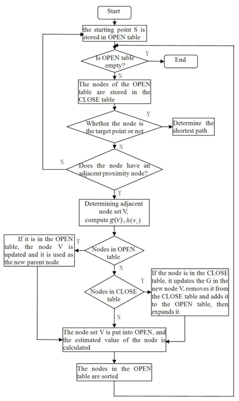
A) Initialize the OPEN table and store starting point S in OPEN.
B) Create the CLOSE table, which is initially empty.
C) Determine whether the OPEN table is empty and exit when it is empty. If not empty, select the OPEN table of the node deleted and stored in the CLOSE table. If the selected point is the target point, exit E, otherwise, select and calculate the adjacent node set V of the node g(v).
D) Determine whether the node is in the OPEN table, and update the G in the node V if it is in the OPEN table, and as a new parent node. If the node is not in the OPEN table, then judge whether it is in the CLOSE, if not in the CLOSE table, then put the node set V into the OPEN table, and calculate the estimated value of the node, and return to C. If the node is in the CLOSE table, update its G value in the new node V, remove it from the CLOSE table, add it to the OPEN table, expand it, and return to C.
E) Sort the last remaining nodes in the OPEN table, and determine the shortest path.
The flow chart of the A* algorithm illustrates that the algorithm relies on the A* heuristic function estimation. However, the process shows that the A* algorithm usually estimates the distance between the target point and the point of state using the Euclidean distance. As a result, a large number of pointless nodes are examined and searched, increasing the algorithm's execution time. Additionally, the repeated traversal of the OPEN table further increases the search time. In this study, an improved A* algorithm based on the weight table query between nodes is proposed to achieve the effective path search, in conjunction with the features of carpool path planning.
2.2.2 Improved A* algorithm based on inter node weight matrix
To eliminate the repeated traversal issue in the A* algorithm’s search process, the A* algorithm based on the weight table query between the link nodes is proposed, that is, the evaluation value of the A* heuristic function is substituted with the weight table between queried nodes. To decrease computation and search time and increase path search efficiency, we can assess the weights of the initial state to the state point and the state point to the target point.
1) Weight matrix between any two nodes
Definition: G=(V,E,W) represents a directed topological network structure in urban road networks, [TeX:] $$V=\{1,2, \cdots n\}$$ represents the set of nodes in a graph, [TeX:] $$E \subseteq V \times V$$ denotes the edge set of the directed topological graph, and W denotes the weight of the directed edges between the nodes i and j. We construct the direct weight matrix (L) of the directed topological graph.
(7)
[TeX:] $$L= \begin{cases}w_{i j} & \left(v_i, v_j\right) \in E, i \neq j \\ 0 & \left(v_i, v_j\right) \in E, i=j \\ \infty & \left(v_i, v_j\right) \notin E\end{cases}$$L denotes the direct weight matrix between the nodes of the directed graph, and [TeX:] $$w_{ij}$$ denotes the weight between nodes i and j. If [TeX:] $$v_i \text { and } v_j$$ are adjacent nodes, the weight is [TeX:] $$w_{ij}$$ If the [TeX:] $$v_i \text { and } v_j$$ are the same nodes, the weight is 0. If the [TeX:] $$v_i \text { and } v_j$$ are non-adjacent nodes, the weights are infinite.
Definition operation rules:
· ⊕ operation rules
The objects of the operation are the two sets [TeX:] $$L_1 \text { and } L_2$$, which are both elements of the set of matrices n×m. This means that [TeX:] $$L_1 \text { and } L_2$$ can be seen as a matrix of numbers in n rows and m columns. The operator symbol is ⊕, and this symbol here represents a specific operation rule, not the traditional addition, subtraction, or multiplication. The result of this operation is another set, [TeX:] $$L_3,$$, which also belongs to the set of n×m matrices. Operation rule: For each corresponding element x(i,j) and y(i,j) in the two sets [TeX:] $$L_1 \text { and } L_2$$, the result of operation ⊕ is to take the smaller value of the two elements, that is, the corresponding element z(i,j) in the set [TeX:] $$L_3,$$ is equal to min(x(i,j),y(i,j)).
· ⊗ operation rules
(11)
[TeX:] $$\vee L_1 \in L^{n \times m}, L_2 \in L^{m \times s}, L_1 \otimes L_2=L_3 \in L^{n \times s}$$
z(i,j) means that the weight of the road is calculated, and each corresponding element x(i,j) and y(i,j) in the two sets [TeX:] $$L_1 \text { and } L_2$$ is multiplied first, and then the minimum value is taken according to the ⊕ operation rule.
· Power operation rule
· The direct weight matrix realizes the minimum weight matrix between any two points by k steps, and obtains the shortest weight matrix [TeX:] $$L_k.$$ After k iteration, the Formula (17) is obtained:
· Any two nodes weight matrix L is defined by Formula (18):
[TeX:] $$L_k$$ represents the shortest weight matrix between any two nodes in a directed graph and is stored in the database as the result of direct query in the heuristic function evaluation of the improved A* algorithm.
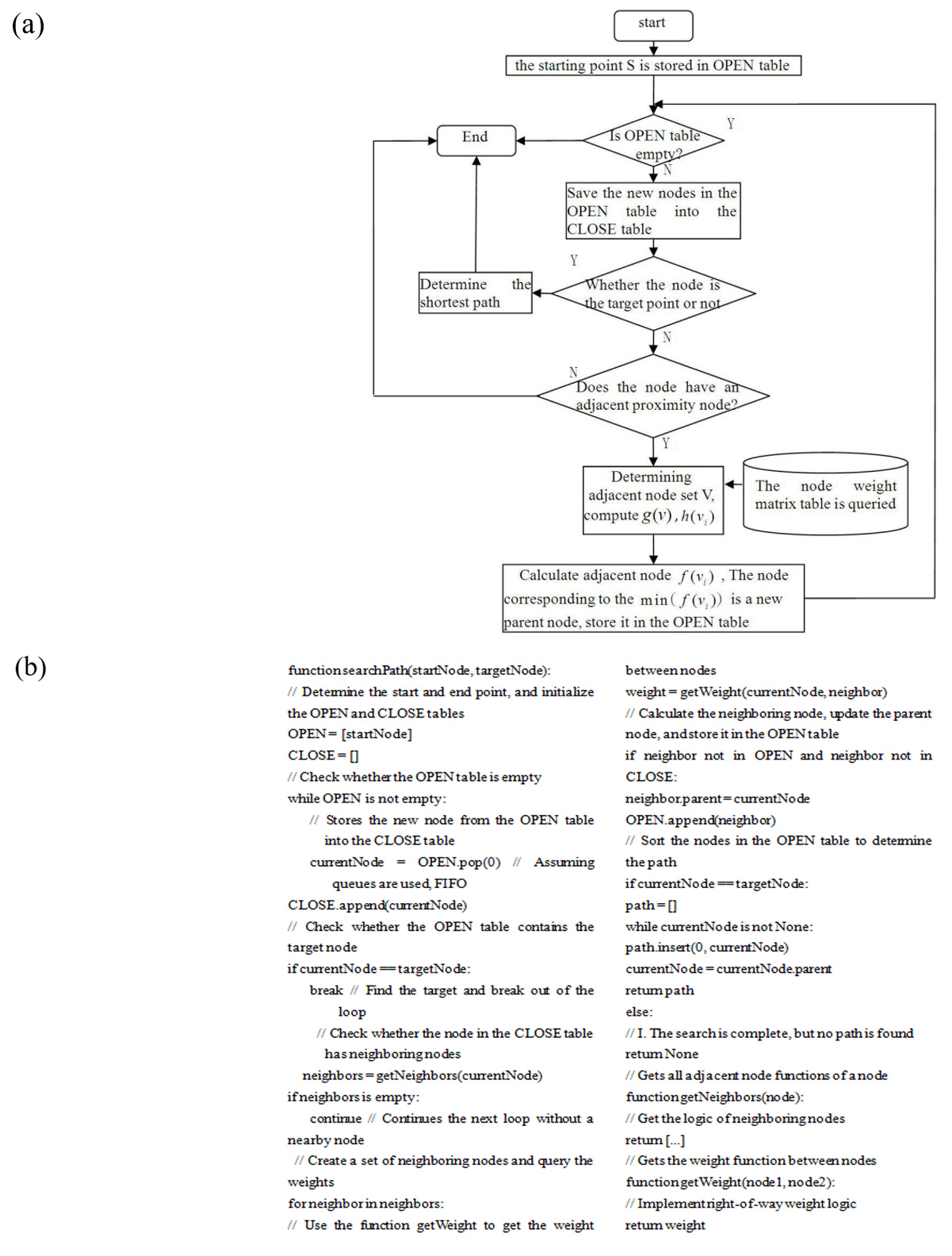
2) Improved A* algorithm flow
Based on node weights, the results of the weight matrix table query between linked nodes are used in the improved A* algorithm to replace the estimated value of the A* heuristic function. The improved algorithm reduces the A* algorithm’s search time and increases path efficiency. The flow chart for the algorithm is displayed in Fig. 2, and the particular steps are as follows:
A) Determine the starting and end points. Starting point S is stored in OPEN, while the CLOSE table is established.
B) Determine whether the OPEN table is empty. If it is empty, then quit to I.
C) Save the new nodes in the OPEN table into the CLOSE table.
D) Determine whether the OPEN table contains the target node. If it does, then go to H; otherwise, go to the next step.
E) If a neighbor node exists in the CLOSE table, go to the next step; otherwise, quit to I.
F) Establish neighbor node set V. The node weight matrix table is called, and the corresponding results of [TeX:] $$g\left(v_1\right), g\left(v_2\right), \ldots, g\left(v_n\right) \text { and } h\left(v_1\right), h\left(v_2\right), \ldots, h\left(v_n\right)$$ in adjacent nodes are searched.
G) Calculate adjacent node [TeX:] $$f\left(v_1\right), i=1,2, \ldots, n .$$ Store the node corresponding to the min[TeX:] $$f\left(v_1\right),$$ which is a new parent node, and store it in the OPEN table. Then, go B.
H) Sort the nodes in the OPEN table and determine the path.
I) End of search.
2.2.3 Comparative analysis of two algorithms
1) The two algorithms differ in the calculation method and search efficiency of the heuristic function estimate.
The core principle of the A* algorithm is to evaluate paths based on the A* heuristic function. The heuristic function f(n) in the A* algorithm typically has two parts, g(n) and h(n), where g(n) is the actual distance between the initial state and state n and h(n) is the optimal path estimated distance between state n and the target state. During the search process, the A* algorithm must calculate the estimated value from each node to the target node, which usually involves calculating the Euclidean distance. Since nodes in the OPEN table must be traversed and evaluated multiple times, the A* algorithm can exhibit prolonged search times when dealing with a large number of nodes.
The improved A* algorithm avoids the repeated computations and node traversals that are present in the A* algorithm’s search procedure. The improved A* algorithm uses the query result of the weight matrix table between the nodes to replace the estimate of the A-inspired function. By calculating and storing the weight matrix between any two nodes beforehand, the improved A* algorithm eliminates the need to calculate Euclidian distance and repeatedly traverse nodes by allowing the weight matrix table to be directly queried during the search process to determine the weight value between nodes. This improvement improves the search efficiency.
2) The difference between the two algorithms in terms of operational efficiency.
Throughout the search process, A* algorithm must determine the estimate from each node to the target node and repeatedly iterate and update the nodes in the OPEN table. When working with a large number of nodes, the A* algorithm may display prolonged search times due to the use of Euclidean distance calculations and repeated node traversals, which results in decreased efficiency.
In contrast, the improved A* algorithm replaces the estimate of the A*inspired function by using the result of the query of the weight matrix table between the nodes, which avoids the calculation of Euclidean distance and repeated traversal of nodes. This improvement enables the improved A* algorithm to find the optimal path faster in the search process, thus improving the operation efficiency. Therefore, the improved A* algorithm is typically more advantageous than the A* algorithm in situations where the shortest path needs to be found quickly.
3. Experimental Analysis
3.1 Experimental Data
In this study, the experimental data for the city taxi in Nanjing on September 16, 2014 after the arrival of the carpool passengers, passengers can carpool taxi matching scheme, as shown in Fig. 3.
Fig. 3 illustrates that P1 and P2 are the starting point and destination of the carpool, respectively. The following taxi numbers are available for carpooling close to P1: 1, 2, 7, 10, 16, 18, 20, 24, 26, and 30. The taxi at destination P2 annex is the destination of the taxi driving near the P1 point. From the point of view of distribution, taxi No.10, No.16, and No. 24 are relatively far away from the destination of P2, and we think the travelling destination near the two taxi and carpool passengers; Taxis at each point are relatively close to the P2 destination, and we think that the taxi and carpool passengers have the same purpose.
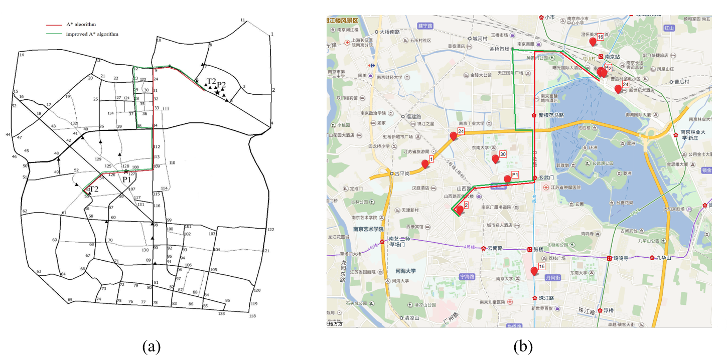
In order to implement carpool path planning, we use the MAPINFO software to digitize the coordinate system and the urban road in Nanjing in Fig. 3, as illustrated in Fig. 4.
Fig. 4 shows that ★ represents the destination and destination of the carpool passenger, and ▲ taxi’s driving point at the P1 annex and the destination of the taxi driving near P2. The thickness of a line in a graph indicates the grade of a road, that is, the thicker the line is, the higher the grade of the road is, and the thinner the line is, the lower the grade of the road is. Taxis 1 to 133 in the figure correspond to road segment node numbers. According to the function of the table in the MAPINFO database, the table structure is established, and the type and range of the related fields are defined, as shown in Table 1.
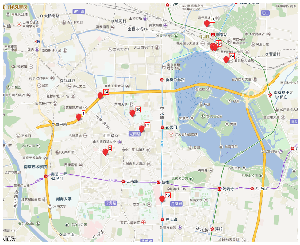
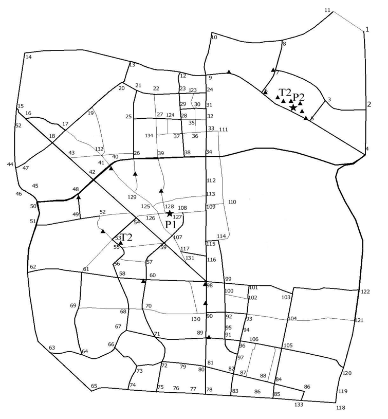
Table 1.
| Route number | Road grade | Origin | Destination | Distance between road nodes (km) | Two way road | Average speed (km/hr) | Waiting time for traffic lights (s) |
|---|---|---|---|---|---|---|---|
| z1 | 2 | 1 | 2 | 1.572 | 111 | 33 | 25 |
| z4 | 2 | 2 | 3 | 0.66 | 111 | 35 | 25 |
| z2 | 2 | 2 | 4 | 0.893 | 111 | 34 | 25 |
| z5 | 2 | 3 | 5 | 0.301 | 111 | 35 | 25 |
| z8 | 2 | 3 | 7 | 1.141 | 111 | 30 | 25 |
| z3 | 2 | 4 | 5 | 1.257 | 111 | 26 | 25 |
| k1 | 1 | 4 | 39 | 2.693 | 111 | 50 | 15 |
| z6 | 2 | 5 | 6 | 1.068 | 111 | 25 | 35 |
| z7 | 2 | 6 | 7 | 0.352 | 111 | 29 | 25 |
| z12 | 2 | 10 | 8 | 1.006 | 111 | 33 | 25 |
| ··· | ··· | ··· | ··· | ··· | ··· | ··· | ··· |
| c43 | 3 | 132 | 26 | 0.359 | 111 | 13 | 45 |
| c41 | 3 | 132 | 41 | 0.279 | 111 | 12 | 45 |
| z143 | 2 | 133 | 118 | 0.454 | 111 | 35 | 25 |
Table 1 presents a city road database table that details various road attributes. The columns in Table 1 are defined as follows: route number indicates the number of each road; road grade indicates the grade of the road, such as the main road and secondary road; origin indicates the area or place where the road starts; destination indicates the area or place where the road ends; distance indicates the distance between the start point and the end point; two way road indicates a two-way road; average speed indicates the average speed of vehicles traveling on this road; and waiting time for traffic lights specifies the average time vehicles spend waiting at traffic lights.
3.2 Experimental Parameters
Table 1 shows that the MAPINFO database table stores the following data: road number, road grade, road length, and road signal waiting time. Using these parameters and the entropy weight method to determine the parameters of the road weight model, we can obtain road weight Formula (19):
The road weight data of the urban road is calculated, and the weight matrix table between any nodes is established, as shown in Table 2.
Table 2 illustrates the weights between any two nodes, with the weight value signifying the strength of the relationship between nodes. By analyzing these weights, we can evaluate nodal connectivity strength and enable the identification of critical nodal junctions or optimal pathways in transportation networks. Due to space limitations, the weight relationship between some nodes is not listed. Therefore, Table 2 uses ellipsis to mark (...). The weights of each node that arrives at its destination can be queried from Table 2. Based on the weights, we can determine the optimal path. This table is used as the basis for improving the A* algorithm to select the intermediate segment in the segment estimation process, and is called directly by the A* algorithm through the database query.
Table 2.
| Nodes\weight | 1 | 2 | 3 | 4 | 5 | ··· | 131 | 132 | 133 |
|---|---|---|---|---|---|---|---|---|---|
| 1 | 30.7642 | 15.3821 | 31.0383 | 30.8433 | 44.3543 | ··· | 134.0918 | 77.0067 | 234.6342 |
| 2 | 15.3821 | 30.7642 | 15.6562 | 15.4612 | 28.9722 | ··· | 118.7097 | 61.6246 | 219.2521 |
| 3 | 31.0383 | 15.6562 | 29.0064 | 29.0739 | 15.5629 | ··· | 132.3224 | 75.2373 | 232.8648 |
| 4 | 30.8433 | 15.4612 | 29.0739 | 27.022 | 13.511 | ··· | 103.2485 | 46.1634 | 203.7909 |
| 5 | 44.3543 | 28.9722 | 15.5629 | 13.511 | 27.022 | ··· | 116.7595 | 59.6744 | 217.3019 |
| 6 | 59.584 | 44.2019 | 28.5457 | 29.1388 | 15.6278 | ··· | 128.3245 | 75.3022 | 232.9297 |
| 7 | 45.5415 | 30.1594 | 14.5032 | 43.1813 | 29.6703 | ··· | 142.367 | 89.3447 | 246.9722 |
| 8 | 32.5458 | 45.2706 | 29.6144 | 58.2925 | 44.7815 | ··· | 143.7641 | 102.1807 | 257.5353 |
| 9 | 61.9384 | 58.1549 | 42.4987 | 43.0918 | 29.5808 | ··· | 114.3715 | 72.7881 | 228.1427 |
| 10 | 47.7807 | 60.5055 | 44.8493 | 57.2495 | 43.7385 | ··· | 128.5292 | 86.9458 | 242.3004 |
| 11 | 16.9218 | 32.3039 | 45.2384 | 47.7651 | 60.4055 | ··· | 151.0136 | 93.9285 | 251.556 |
| 12 | 75.7266 | 71.9431 | 56.2869 | 56.88 | 43.369 | ··· | 100.5833 | 58.9999 | 222.0973 |
| 13 | 89.8853 | 86.1018 | 70.4456 | 71.0387 | 57.5277 | ··· | 86.4246 | 44.8412 | 207.9386 |
| ··· | ··· | ··· | ··· | ··· | ··· | ··· | ··· | ··· | ··· |
| 129 | 76.322 | 60.9399 | 74.5526 | 45.4787 | 58.9897 | ··· | 70.6381 | 29.3953 | 192.1521 |
| 130 | 152.687 | 137.3049 | 150.9176 | 121.8437 | 135.3547 | ··· | 29.7988 | 100.0573 | 106.4913 |
| 131 | 134.0918 | 118.7097 | 132.3224 | 103.2485 | 116.7595 | ··· | 27.2144 | 70.2585 | 121.514 |
| 132 | 77.0067 | 61.6246 | 75.2373 | 46.1634 | 59.6744 | ··· | 70.2585 | 29.5272 | 191.7725 |
| 133 | 234.6342 | 219.2521 | 232.8648 | 203.7909 | 217.3019 | ··· | 121.514 | 191.7725 | 31.0482 |
3.3 Experimental Result Analysis
3.3.1 Quantitative comparison of algorithm efficiency
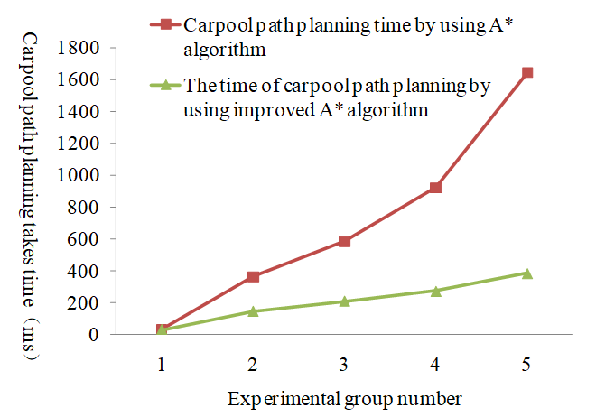
When determining the shortest path between the starting and end points, the traditional A* algorithm and other extended A* algorithms (like the bidirectional A* algorithm, multi-level landmark based A* algorithm, etc.) mainly consider distance. These algorithms will also look into and search some useless nodes during the calculation, which will make the algorithm run too long. Road segment length, vehicle speed within road nodes, road grade, and traffic light impact are the factors that the algorithm presented in this paper uses to create a road weight function. This function generates road weight values, which are stored in a database. In the improved A* algorithm, the road weight value of the sorted nodes can be directly sorted to obtain the optimal path and reduce the running time of the algorithm. In the experiment, we randomly selected five sets of data on the destination to destination distance in the map: 1 km, 3 km, 6 km, 10 km, and 15 km. Based on this data, we use algorithm A* and improved A* algorithm for path planning.
Table 3.
| Place of departure | Destination | Distance (km) | Algorithm time (ms) | |||
|---|---|---|---|---|---|---|
| Longitude | Latitude | Longitude | Latitude | A* | Improved A* | |
| 118.7788 | 32.0545 | 118.7809 | 32.0438 | 1 | 33 | 31 |
| 118.7729 | 32.0613 | 118.7681 | 32.0355 | 3 | 361 | 146 |
| 118.7787 | 32.0587 | 118.7163 | 32.0391 | 6 | 583 | 210 |
| 118.7068 | 32.0019 | 118.7675 | 32.0823 | 10 | 921 | 272 |
| 118.7947 | 32.0993 | 118.7475 | 31.9775 | 15 | 1640 | 384 |
To compare the A* algorithm with the proposed algorithm, the effectiveness of the proposed algorithm is verified using VB6.0 to write two algorithms. We conduct experimental verification in the WINXP system on a 3.1 GHZ main frequency, 2.9 GB memory platform.
Table 3 demonstrates that the improved A* algorithm exhibits shorter computation times than the traditional A* algorithm. This is due to the fact that the traditional A* algorithm usually calculates the Euclidean distance between the target point and the current state. The traditional A* algorithm inspects and searches for many useless nodes, thereby extending the run time. To show the contrast effect clearly, a time-consuming contrast diagram between A* algorithm and improved A* algorithm is established, as shown in Fig. 5.
The path planning and travel time of five groups of experimental data are computed using the traditional A* algorithm and the improved A* algorithm, respectively, based on the length of road nodes, the traffic light waiting time, and the average driving speed of vehicles in Table 1. Since the traditional A* algorithm relies solely on distance for path calculations, whereas the improved A* algorithm incorporates comprehensive road weights. It can be seen from Table 4 that the improved A* algorithm is superior to the traditional A* algorithm in travel time. Especially in the upper distance travel, the improved A* algorithm is obviously superior to the traditional A* algorithm.
Table 4.
| Place of departure | Destination | Distance (km) | Algorithm time (ms) | |||
|---|---|---|---|---|---|---|
| Longitude | Latitude | Longitude | Latitude | A* | Improved A* | |
| 118.7788 | 32.0545 | 118.7809 | 32.0438 | 1 | 2.7 | 2.7 |
| 118.7729 | 32.0613 | 118.7681 | 32.0355 | 3 | 7.4 | 7.1 |
| 118.7787 | 32.0587 | 118.7163 | 32.0391 | 6 | 16.9 | 15.7 |
| 118.7068 | 32.0019 | 118.7675 | 32.0823 | 10 | 21.5 | 19.3 |
| 118.7947 | 32.0993 | 118.7475 | 31.9775 | 15 | 33.6 | 30.1 |
3.3.2 Empirical comparison of algorithms
By comparing the A* algorithm and the improved A* algorithm under the same test environment and conditions, the improved A* algorithm is superior to the traditional A* algorithm in computing efficiency and time dimension, which proves the effectiveness of the proposed algorithm in considering time cost. In order to further verify the practical applicability of the proposed algorithm, this paper selected the No. 2 taxi from the experimental data, and used the two algorithms to plan and calculate the combined route, and obtained the calculation results as shown in Fig. 6.
The variations in route selection between the two algorithms are shown in Fig. 6. According to the road vector diagram, the driving path of the traditional A* algorithm can be seen as follows: 55→53→54→126→127→108→109→34→33→32→31→24→9→6, the driving distance is 5.045 km, and the driving time is about 24 minutes. The driving path of the improved A* algorithm is: 55→53→54→126→127→108→109→34→38→28→23→12→9→6, the driving distance is 5.667 km, and the driving time is about 21 minutes. In terms of time cost, the algorithm proposed in this paper is superior to the traditional A* algorithm, because the traditional A* algorithm only considers the shortest path in the path planning process, and does not consider the actual situation of the road. The algorithm proposed in this paper no longer takes the distance or time as the basic path planning index. Instead, the dynamic road traffic information obtained in real time in the city, such as road length, vehicle speed on node roads, road grade and traffic lights in the road, is calculated by the road weight function and its road weight value is used as the path planning index to realize the path re-planning after the city taxis share the ride. Therefore, the improved A* algorithm turns out to be more efficient in terms of both time efficiency and practical application.
5. Conclusion
The network topology of urban roads is constructed by the layer method, an electronic map is established, and the urban road network database is constructed. We calculated the road weights of the data on the road network database using the road weighting function, combined the improved A* algorithm to determine the weight table between nodes and achieved a carpool path planning.
Using VB6.0 and MAPINFO, we created the urban taxi ride path planning simulation experiment platform based on the improved A* algorithm model. According to the simulation results, the suggested algorithm can be a useful guide for taxi drivers and carpool passengers when it comes to planning the best routes.
Future studies will further optimize the road weight index and offer a useful reference for carpooling passengers by combining the findings of this study with other factors that affect taxi carpooling, such as cost, distance, load balance between passengers, etc., to investigate the application of multi-objective optimization (e.g., time and cost) or combined objective function.
Funding
This paper is supported by the National Natural Science Foundation of China (Grant No. 52062026 and 52162041) and Educational Commission of Gansu Province of China (Grant No. 2019A-041) and Double-First Class Major Research Programs, Educational Department of Gansu Province (No. GSSYLXM-04) and top Talent Program for Basic Research of Lanzhou Jiaotong University (No. 2022JC56).
Biography
Qiang Xiao
https://orcid.org/0000-0002-6696-7041
He received M.S. degrees in School of electronic information and electrical engineering from Lanzhou Jiaotong University in 2007, and Ph.D. degree in School of Traffic and Transportation from Lanzhou Jiaotong University in 2017. He is currently a professor in School of Economics and Management, Lanzhou Jiaotong University, Gansu, China. His research interests include data mining and data analysis.
Biography
Biography
References
- 1 Q. Xiao, R. He, and C. Ma, "The analysis of urban taxi carpooling impact from taxi GPS data," Archives of Transport, vol. 47, no. 3, pp. 109-120, 2018. https://doi.org/10.5604/01.3001.0012.6514doi:[[[10.5604/01.3001.0012.6514]]]
- 2 S. Gao, J. Y . Yang, X. J. Wu, and T. Ming, "Solving circle permutation problem with ant colony-simulated annealing algorithm," Systems Engineering: Theory and Practice, vol. 24, no. 8, pp. 102-106, 2004. https://sysengi.cjoe.ac.cn/EN/10.12011/1000-6788(2004)8-102doi:[[[https://sysengi.cjoe.ac.cn/EN/10.12011/1000-6788(2004)8-102]]]
- 3 G. Barbarosoglu and D. Ozgur, "Hierarchical design of an integrated production and 2-echelon distribution system," European Journal of Operational Research, vol. 118, no. 3, pp. 464-484, 1999. https://doi.org/ 10.1016/S0377-2217(98)00317-8doi:[[[10.1016/S0377-2217(98)00317-8]]]
- 4 S. Jung and S. Pramanik, "An efficient path computation model for hierarchically structured topographical road maps," IEEE Transactions on Knowledge and Data Engineering, vol. 14, no. 5, pp. 1029-1046, 2002. https://doi.org/10.1109/TKDE.2002.1033772doi:[[[10.1109/TKDE.2002.1033772]]]
- 5 R. Bauer, D. Delling, P. Sanders, D. Schieferdecker, D. Schultes, and D. Wagner, "Combining hierarchical and goal-directed speed-up techniques for Dijkstra’s algorithm," Journal of Experimental Algorithmics (JEA), vol. 15, article no. 2.3, 2010. https://doi.org/10.1145/1671970.1671976doi:[[[10.1145/1671970.167]]]
- 6 R. Rajagopalan, K. G. Mehrotra, C. K. Mohan, and P. K. Varshney, "Hierarchical path computation approach for large graphs," IEEE Transactions on Aerospace and Electronic Systems, vol. 44, no. 2, pp. 427-440, 2008. https://doi.org/10.1109/TAES.2008.4560197doi:[[[10.1109/TAES.2008.4560197]]]
- 7 Q. Song and X. Wang, "Efficient routing on large road networks using hierarchical communities," IEEE Transactions on Intelligent Transportation Systems, vol. 12, no. 1, pp. 132-140, 2011. https://doi.org/10.1109/ TITS.2010.2072503doi:[[[10.1109/TITS.2010.503]]]
- 8 S. Nordbeck and B. Rystedt, Computer Cartography: Shortest Route Programs. Lund, Sweden: Royal University of Lund, 1969.custom:[[[-]]]
- 9 S. C. Hirtle and J. Jonides, "Evidence of hierarchies in cognitive maps," Memory & Cognition, vol. 13, no. 3, pp. 208-217, 1985. https://doi.org/10.3758/BF03197683doi:[[[10.3758/BF0383]]]
- 10 A. Car and A. Frank, "General principles of hierarchical spatial reasoning-the case of wayfinding," in Proceedings of the 6th International Symposium on Spatial Data Handling, Edinburgh, Scotland, 1994, pp. 646-664.custom:[[[-]]]
- 11 P. Sanders and D. Schultes, "Highway hierarchies hasten exact shortest path queries," in Algorithms – ESA 2005. Berlin, Heidelberg: Springer, 2005, pp. 568-579. https://doi.org/10.1007/11561071_51doi:[[[10.1007/11561071_51]]]
- 12 M. F. Goodchild, "GIS and transportation: status and challenges," GeoInformatica, vol. 4, pp. 127-139, 2000. https://doi.org/10.1023/A:1009867905167doi:[[[10.1023/A:1009867905167]]]
- 13 P. Sanders and D. Schultes, "Engineering highway hierarchies," Journal of Experimental Algorithmics (JEA), vol. 17, article no. 1.6, 2012. https://doi.org/10.1145/2133803.2330080doi:[[[10.1145/803.2330080]]]
- 14 V . Maniezzo and A. Colorni, "The ant system applied to the quadratic assignment problem," IEEE Transactions on Knowledge and Data Engineering, vol. 11, no. 5, pp. 769-778, 1999. https://doi.org/10.1109/ 69.806935doi:[[[10.1109/69.806935]]]
- 15 M. Dorigo and L. M. Gambardella, "Ant colony system: a cooperative learning approach to the traveling salesman problem," IEEE Transactions on Evolutionary Computation, vol. 1, no. 1, pp. 53-66, 1997. https://doi.org/10.1109/4235.585892doi:[[[10.1109/4235.585892]]]
- 16 M. Dramski, "A comparison between Dijkstra algorithm and simplified ant colony optimization in navigation," Zeszyty Naukowe (Scientific Journal), vol. 29, no. 101, pp. 25-29, 2012. https://repository.am. szczecin.pl/handle/123456789/422doi:[[[https://repository.am.szczecin.pl/handle/123456789/422]]]
- 17 Z. Cong, B. De Schutter, and R. Babuska, "Ant colony routing algorithm for freeway networks," Transportation Research Part C: Emerging Technologies, vol. 37, pp. 1-19, 2013. https://doi.org/10.1016/ j.trc.2013.09.008doi:[[[10.1016/j.trc.2013.09.008]]]
- 18 P. Du, X. Bai, K. Tan, Z. Xue, A. Samat, J. Xia, E. Li, H. Su, and W. Liu, "Advances of four machine learning methods for spatial data handling: a review," Journal of Geovisualization and Spatial Analysis, vol. 4, article no. 13, 2020. https://doi.org/10.1007/s41651-020-00048-5doi:[[[10.1007/s41651-020-00048-5]]]
- 19 X. Yu, V . A. van den Berg, and E. T. Verhoef, "Carpooling with heterogeneous users in the bottleneck model," Transportation Research Part B: Methodological, vol. 127, pp. 178-200, 2019. https://doi.org/10.1016/j.trb. 2019.07.003doi:[[[10.1016/j.trb.2019.07.003]]]
- 20 Q. Xiao, R. He, C. Ma, and W. Zhang, "Evaluation of urban taxi-carpooling matching schemes based on entropy weight fuzzy matter-element," Applied Soft Computing, vol. 81, article no. 105493, 2019. https://doi.org/10.1016/j.asoc.2019.105493doi:[[[10.1016/j.asoc.2019.105493]]]
- 21 M. Tamannaei and I. Irandoost, "Carpooling problem: a new mathematical model, branch-and-bound, and heuristic beam search algorithm," Journal of Intelligent Transportation Systems, vol. 23, no. 3, pp. 203-215, 2019. https://doi.org/10.1080/15472450.2018.1484739doi:[[[10.1080/15472450.2018.1484739]]]
- 22 H. Huang, D. Bucher, J. Kissling, R. Weibel, and M. Raubal, "Multimodal route planning with public transport and carpooling," IEEE Transactions on Intelligent Transportation Systems, vol. 20, no. 9, pp. 35133525, 2019. https://doi.org/10.1109/TITS.2018.2876570doi:[[[10.1109/TITS.2018.2876570]]]
- 23 X. Liu, H. Titheridge, X. Yan, R. Wang, W. Tan, D. Chen, and J. Zhang, "A passenger-to-driver matching model for commuter carpooling: case study and sensitivity analysis," Transportation Research Part C: Emerging Technologies, vol. 117, article no. 102702, 2020. https://doi.org/10.1016/j.trc.2020.102702doi:[[[10.1016/j.trc.2020.102702]]]
- 24 J. Wang, H. Wang, and X. Yu, "Parking permit management of morning commuting considering carpooling with parking restraint," Journal of Transportation Engineering, Part A: Systems, vol. 146, no. 7, article no. 04020052, 2020. https://doi.org/10.1061/JTEPBS.0000368doi:[[[10.1061/JTEPBS.0000368]]]