Research on Maximum Power Point Tracking Algorithms for Photovoltaic Cells

1. Introduction

With the global increase in energy consumption, an increasing number of countries have realized that relying solely on fossil fuels, such as oil and coal, is not a long-term solution [1]. Energy-saving and environmentally friendly power generation technologies have attracted considerable attention, and solar energy, which is abundant, clean, and green, has become the first choice for countries to explore and develop [2].

Photovoltaic (PV) cells are crucial components in PV power generation systems. Their output power exhibits significant nonlinear characteristics under different environmental conditions, such as sunlight and temperature [3]. However, under fixed environmental conditions, they show a unique maximum power point [4]. Because the environment is not constant, continuous optimization and improvement in maximum power point tracking (MPPT) algorithms are required to minimize power losses and ensure that PV cells operate as close to the maximum power point as possible [5].

In this study, the output characteristics of PV cells and their characteristic curves under different temperatures or sunlight levels were investigated based on the principles of PV power generation and commonly used engineering mathematical models. This paper provides a detailed introduction to the principles of Boost circuits involved in MPPT [6]. Furthermore, it elaborates on the principles and advantages/disadvantages of the perturb-and-observe, incremental conductance, and constant voltage methods used in MPPT. Finally, utilizing a simulation model established in MATLAB Simulink, this study analyzed these three MPPT algorithms. The simulation results were compared with relevant theories to verify the accuracy of the simulation [7].

The remainder of this paper is organized as follows. Section 2 presents a brief review of the mathematical model of a PV cell. The PV cell output characteristics and analysis of the influencing factors are described in Section 3. Section 4 presents the principles and methods of MPPT. Experimental results for the proposed method are presented in Section 5. Finally, conclusions and remarks on possible future work are presented in Section 6.

2. Photovoltaic Cell Mathematical Model

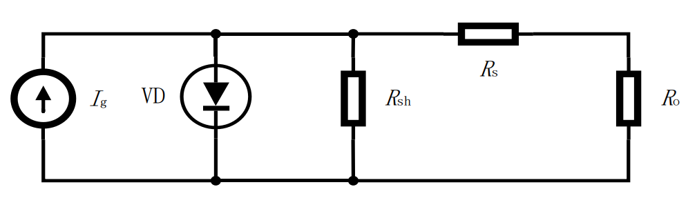
The equivalent circuit of a PV cell is depicted in Fig. 1. [TeX:] $$I_g$$ represents the photocurrent generated by the PV array, which is approximately proportional to the intensity of sunlight. [TeX:] $$I_d$$ denotes the reverse current of the equivalent diode, [TeX:] $$R_{\mathrm{sh}}$$ denotes the internal equivalent parallel resistance of the photovoltaic cell, [TeX:] $$R_{\mathrm{s}}$$ represents the series resistance, and [TeX:] $$I_{\mathrm{sh}}$$ is the current flowing through the equivalent parallel resistance. Therefore, the expression for the voltage-current characteristic is given by Eq. (1):

where [TeX:] $$I_d \text { and } I_{\mathrm{sh}}$$ are expressed by Eqs. (2) and (3), respectively.

In Eq. (2), [TeX:] $$I_{\mathrm{sat}}$$ represents the reverse saturation current of the diode, where q represents the electron charge [TeX:] $$\left(q=1.6 \times 10^{-19} \mathrm{C}\right), V_o$$ s the output voltage of the PV cell, A is the diode ideality factor, K is the Boltzmann constant [TeX:] $$\left(K=1.38065 \times 10^{-23} \mathrm{~J} / K\right), \text { and } T$$ is the absolute temperature (in Kelvin). The PV cell model adopted in this study was the engineering practical [TeX:] $$C_1 C_2$$ mathematical model. This model assumes that the equivalent parallel resistance [TeX:] $$R_{\mathrm{sh}}$$ is very large; thus, ignoring [TeX:] $$I_{\mathrm{sh}}$$ in Eq. (1), the forward conducting resistance of the diode is much greater than [TeX:] $$R_{\mathrm{sh}}$$, and the short-circuit current [TeX:] $$I_{\mathrm{sc}}$$ of the PV array equals the photocurrent [TeX:] $$I_g$$ of the PV array.

Under standard test conditions for PV modules on the ground, the current–voltage equation for a solar cell can be derived from Eqs. (1)–(3) as

where constants [TeX:] $$C_1 \text { and } C_2$$ are given by,

respectively, where [TeX:] $$V_{\mathrm{oc}}$$ is the open-circuit voltage of the PV array, [TeX:] $$I_m$$ is the maximum power point current, and [TeX:] $$V_m$$ is the maximum power point voltage in Eqs. (4)–(6)

Under the standard test conditions of non-terrestrial PV modules, i.e., when the light temperature changes, Eq. (4) can be corrected according to Eq. (7):

where [TeX:] $$D_I \text { and } D_V$$ represent the changes in illumination R and temperature [TeX:] $$T_a,$$ respectively, with the expressions for the output current and voltage of the PV array given by

respectively, where α is the temperature coefficient of the PV array’s current, [TeX:] $$R_{\mathrm{ref}}$$ is the light intensity under standard conditions [TeX:] $$\left(R_{\mathrm{ref}}=1,000 \mathrm{~W} / \mathrm{m}^2\right), \beta$$ is the temperature coefficient of voltage, and [TeX:] $$D_T$$ is the difference between the actual temperature [TeX:] $$T_c$$ and standard temperature, as follows:

where [TeX:] $$T_{\text {ref }}$$ is the temperature under standard conditions [TeX:] $$\left(T_{\mathrm{ref}}=25^{\circ} \mathrm{C}\right), T_c$$ is the ambient temperature, and [TeX:] $$T_a$$ is the real-time light intensity. The relationship between these is expressed by

where γ is the temperature coefficient of module temperature rise.

3. Photovoltaic Cell Output Characteristics and Analysis of Influencing Factors

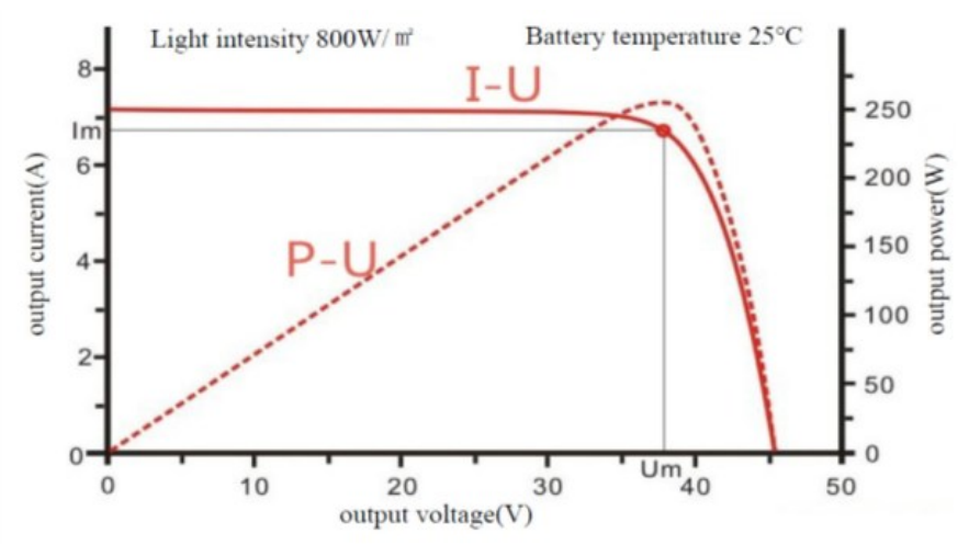
By analyzing the mathematical model of PV cells, as shown in Fig. 1, the output voltage and current of PV cells continuously change with variations in the light intensity and temperature characteristics. The output characteristic curve of the PV cell at a light intensity of 800 W/m² and cell temperature of [TeX:] $$25^{\circ} \mathrm{C}$$ is shown in Fig. 2. The solid line represents the I-U curve of the PV cell, where the voltage remains relatively constant within the range of [TeX:] $$0-U_m$$ and gradually decreases as it approaches [TeX:] $$U_m.$$ The dashed line represents the curve of the PV cell’s power output P-U, which is a single-peak curve. The power increases continuously in the voltage range of [TeX:] $$0-U_m$$ and reaches its maximum value at [TeX:] $$U_m,$$ which is the maximum power point of the PV cell. [TeX:] $$I_m \text { and } U_m$$ denote the current and voltage at the maximum power point, respectively, whereas [TeX:] $$P_m$$ represents the maximum output power, expressed as

3.1 Illumination Characteristics

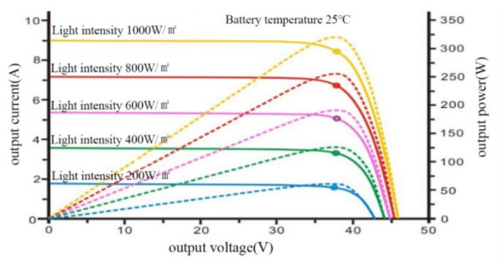
Light intensity is an important factor that affects the maximum power point. The characteristic curves of PV cells at a fixed temperature of [TeX:] $$25^{\circ} \mathrm{C}$$ are shown in Fig. 3. The solid line represents the I-U curve. As the light intensity increases from 200 W/m² to 1,000 W/m², the short-circuit current is significantly influenced, increasing from approximately 1.9 to 9 A. The dashed line represents the P-U curve. The open-circuit voltage is less affected by the light intensity, with a small increase. The maximum output power also increases, from 50 W to 300 W. Therefore, light intensity is an important factor to consider when studying MPPT.

3.2 Temperature Characteristics

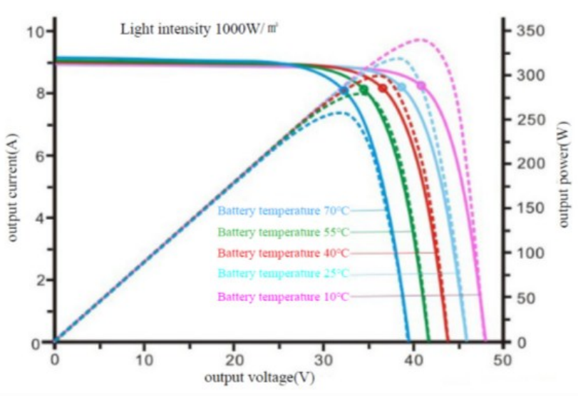
The temperature of the environment in which PV cells are located is also an important factor affecting the maximum power point. Under a light intensity of 1,000 W/m², the I–V and P–V characteristics at different cell temperatures are depicted in Fig. 4. The solid line represents the I–V characteristic curve. As the cell temperature increases from [TeX:] $$10^{\circ} \mathrm{C} \text { to } 70^{\circ} \mathrm{C}$$, the open-circuit voltage decreases, dropping from approximately 48 V to 40 V. The dashed line represents the P–V characteristic curve. With increasing temperature, the short-circuit current slightly increases, but its magnitude is small. The output power also increases. When the cell temperature is [TeX:] $$10^{\circ} \mathrm{C}$$, the maximum output power is 340 W, whereas when the cell temperature is [TeX:] $$70^{\circ} \mathrm{C}$$, the maximum output power is 250 W.

4. Principle and Methods of Maximum Power Point Tracking

As the temperature of the cells decreases or light intensity increases, the output power of PV cells increases. However, only one maximum power point exists under certain illumination and temperature conditions. To further improve the photoelectric conversion efficiency, tracking the maximum power point of PV cells is necessary.

4.1 Boost Circuit Principle

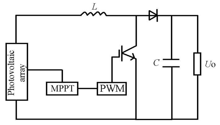
To achieve MPPT of PV cells, a converter capable of performing this function must be added to the PV power generation system. To achieve optimal results, power converters generally employ a combination of DC/DC with Boost conversion circuits. The Boost conversion circuit used is depicted in Fig. 5. When all components in the circuit are in the ideal states, the relationship between the input and output voltages, as well as the input and output currents, is governed by Eqs. (13) and (14), respectively.

where D represents the duty cycle of the power switch, and the equivalent input impedance of the circuit is expressed as Eq. (15):

In the Boost converter, if the impedance of the actual load remains constant, changing the duty cycle D can alter the equivalent input impedance represented by [TeX:] $$R_{\mathrm{in}},$$ thereby causing a change in the output current of the PV cells. Consequently, the operating point and output power of the PV array change accordingly. By controlling the duty cycle of the power converter according to specific control laws, PV cells operate at or very close to the maximum power point under specific conditions, thereby tracking the maximum power point of the PV system.

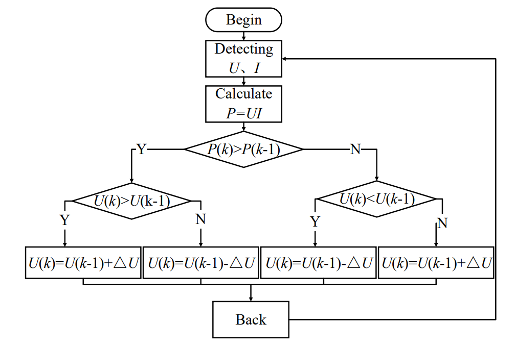
4.2 Perturbation and Observation Method

The perturbation and observation method (P&O), which is known as the hill-climbing method, is widely used in various industries. When [TeX:] $$\Delta P / \Delta U=0,$$ it achieves the maximum power point [TeX:] $$P_m .$$ As illustrated in Fig. 6, the process flowchart of the perturbation observation method, the output power at this moment is represented by [TeX:] $$P_k,$$ where [TeX:] $$P_{k-1}$$ represents the output power of the previous moment. The principle of MPPT with P&O can be described as follows: continuously applying a voltage increment [TeX:] $$\Delta U,$$ i.e., perturbing the output voltage. By detecting the output voltage and current to calculate the output power P, the sizes of the previous and current output powers, [TeX:] $$P_k \text{ and } P_{k-1},$$ are compared. If the power at this moment, [TeX:] $$P_k,$$ is greater, this indicates that the perturbation direction is correct and that the perturbation should continue in this direction. If [TeX:] $$P_k$$ is smaller, the perturbation direction is incorrect, and the perturbation should be in the opposite direction. By continuously perturbing the output voltage in this manner, it operates near the maximum power point.

The advantages of P&O include its simple principle, relatively few measured parameters, high conversion efficiency, and ease of implementation. However, its disadvantages include the inability to operate stably at the maximum power point; it can only oscillate near the maximum power point, inevitably leading to power loss. The size of the perturbation step, i.e., the increment in voltage, significantly affects control precision and speed. It also exhibits poor responsiveness to environmental changes; sudden changes in illumination may result in incorrect perturbation directions. Therefore, this method is only suitable for environments with small variations in light intensity.

4.3 Incremental Conductance Method

The principle of the incremental conductance method is to determine the maximum power point by calculating and comparing the instantaneous conductance and change in conductance of the solar cell. According to the PV characteristic curve, only one maximum power point [TeX:] $$P_m$$ exists on the curve, where the slope of the characteristic curve is zero, indicating [TeX:] $$\frac{d P}{d U}=0 .$$ The power formula is

According to the rules of differential calculus, following can be deduced at the maximum power point,

when [TeX:] $$U\lt U_m, \frac{d P}{d U}\gt 0,$$ implying [TeX:] $$\frac{d I}{d U}\gt -\frac{I}{U} ;$$ when [TeX:] $$U\gt U_m, \frac{d P}{d U}\lt 0,$$ implying [TeX:] $$\frac{d I}{d U}\lt -\frac{I}{U}.$$

The incremental conductance method employs [TeX:] $$U_{tk}$$ to represent the updated voltage value after calculation. First, dU and dI are determined to be zero or not. If both are zero, the PV cell is already operating at the maximum power point, and the output voltage should remain unchanged. If dU is zero and dI is non-zero, the value can be determined by the sign of dI. If dU is non-zero, [TeX:] $$U_{tk}$$ is determined based on whether Eq. (18) holds true, i.e., whether the change in conductance is equal to the negative value of the output conductance.

The advantage of the incremental conductance method is that when the illumination and temperature change, the PV array will stabilize near the maximum power point. It offers precise control and fast tracking speed, effectively reduces power loss, and improves conversion efficiency. However, its disadvantage lies in its complexity, as it requires relatively high-precision hardware, such as sensors and controllers, leading to higher costs and making it difficult to implement in engineering applications

4.4 Constant Voltage Method

From the characteristic curves in Fig. 2, when the temperature is constant, the maximum power points of each curve are generally near a vertical line. Once this vertical line is found, the voltage value [TeX:] $$U_m$$ (approximately 0.78 times the open-circuit voltage) can be determined. By comparing the sampled voltage U with the reference voltage [TeX:] $$U_m$$, the duty cycle D is adjusted to maintain the output voltage of the battery panel at [TeX:] $$U_m$$. This simplifies the MPPT control to voltage regulation, allowing the PV battery to operate at the maximum power point.

The advantages of using the constant voltage method (CVT) to achieve MPPT of PV batteries are that the control is simple and easy to implement, the stability is relatively high, and it can be realized through software and hardware. However, setting the system operating voltage is relatively challenging, because the ambient temperature has a significant impact on the open-circuit voltage, and improper settings can easily lead to efficiency loss [8]. It is more suitable for small-scale PV systems in areas with relatively stable temperature changes and light conditions.

5. MPPT Algorithm Simulation Analysis

To deepen our understanding and differentiation of the three MPPT methods, this study used MATLAB Simulink to build a generic module for PV batteries in which the main parameters of maximum output power, voltage, and current are [TeX:] $$P_m=140.5 \mathrm{~W}, V_m=17.7 \mathrm{~V}, \text { and } I_m=7.94 \mathrm{~A} .$$ Using the MPPT module to implement algorithm control, the output reference voltage was compared with the carrier wave to generate pulse width modulation (PWM) waves, and the PWM was used to drive the Boost circuit to switch on and off to adjust the duty cycle, thereby finding the maximum power point and tracking it.

This simulation circuit model uses a combination of a signal generator and switch to freely create four operating modes: Mode 1, fixed temperature, fixed light intensity; Mode 2, fixed temperature, sudden change in light intensity; Mode 3, sudden change in temperature, fixed light intensity; Mode 4, sudden change in temperature, sudden change in light intensity. The simulation results were analyzed and compared.

5.1 Disturbance Observation Method Simulation Analysis

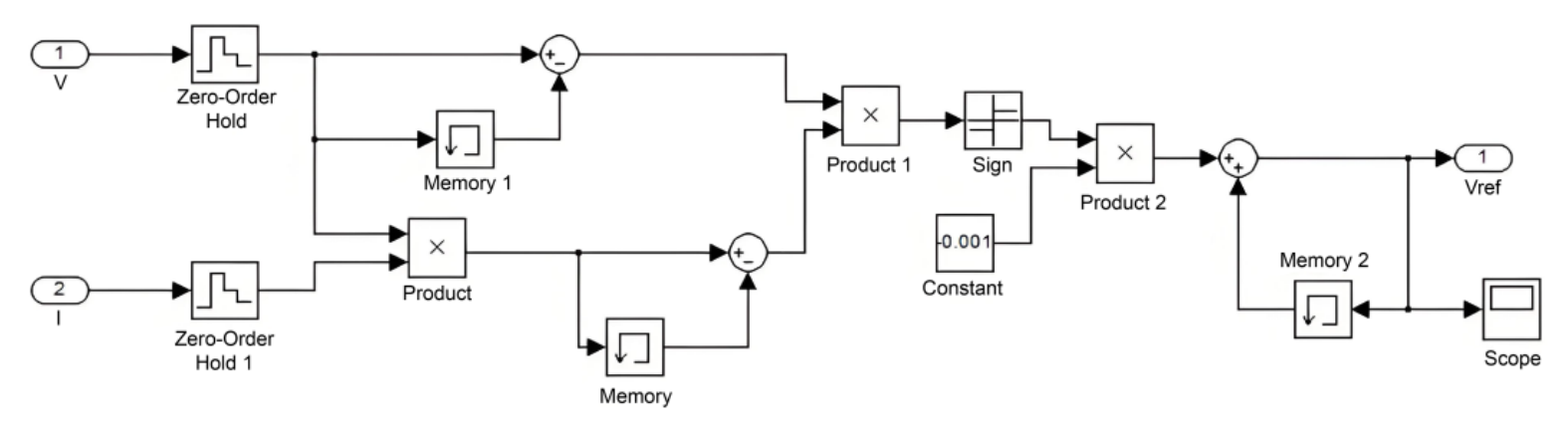
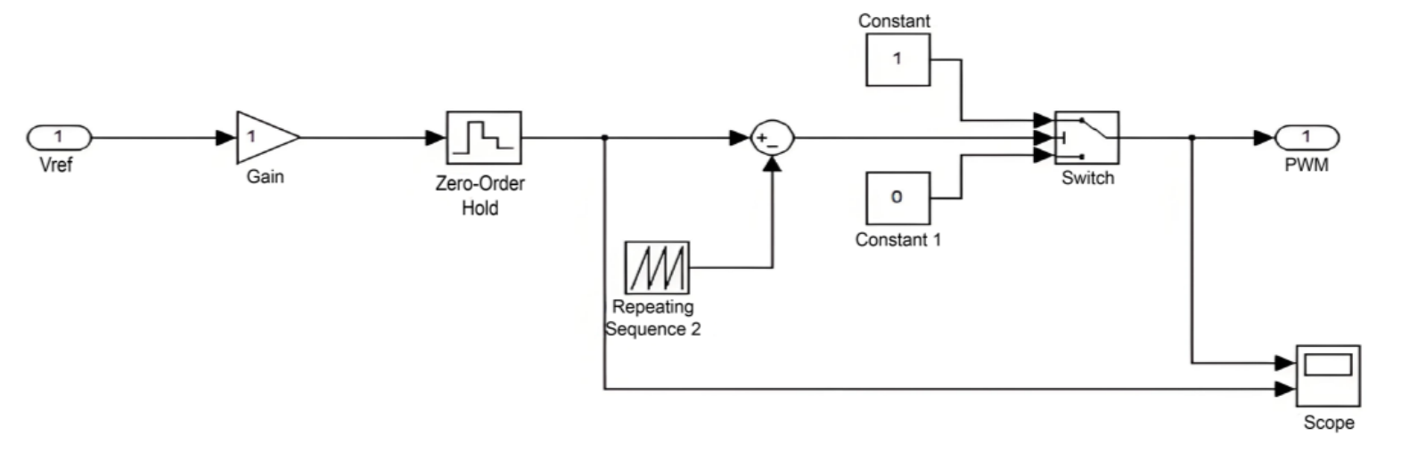
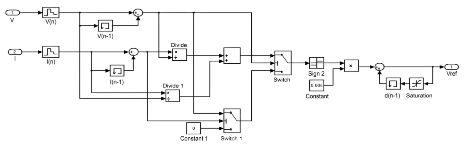
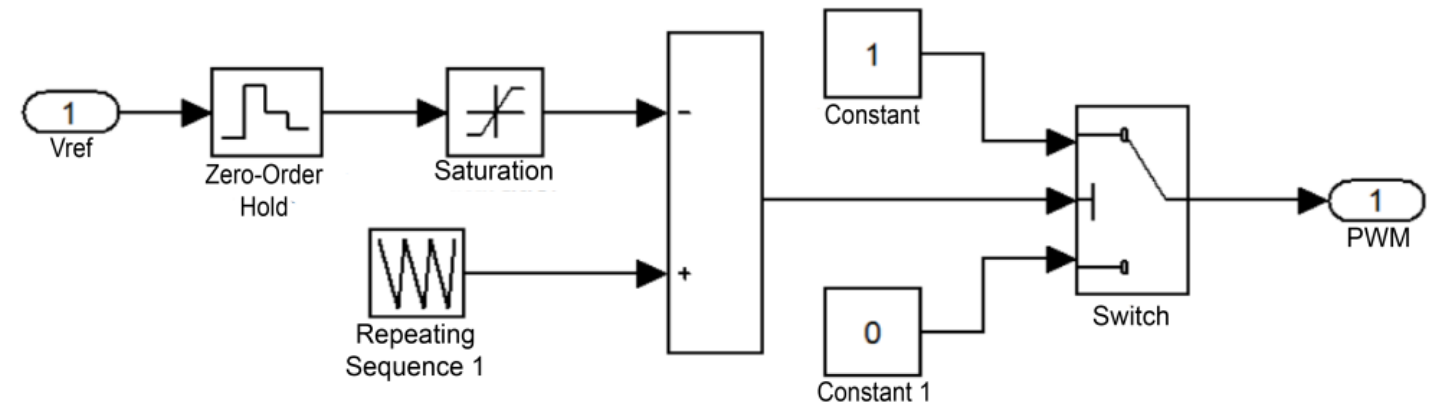
As shown in Fig. 7, the disturbance observation MPPT module processes the input voltage and current through a series of calculations. The module outputs the duty cycle at the current moment. Subsequently, the PWM module, as depicted in Fig. 8, determines the conduction or disconnection of the Boost circuit to track the maximum power point.

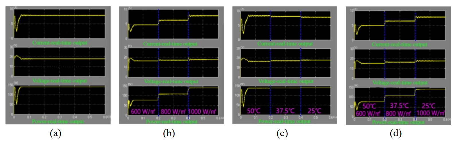
As shown in Fig. 9(a), using the disturbance observation method, under conditions of [TeX:] $$25^{\circ} \mathrm{C}$$ temperature and 1,000 W/m² illumination intensity, the maximum power tracking was completed in approximately 0.03 seconds. Fig. 9(b) illustrates that with a fixed environmental temperature, as the illumination intensity increased from 600 W/m² to 1,000 W/m², the output current significantly increased, whereas the output voltage slightly increased, increasing the output power. From Fig. 9(c), with a constant environmental illumination intensity, as the environmental temperature decreased, the output voltage increased, and the output current slightly decreased, increasing the maximum power. Fig. 9(d) shows that when environmental temperature decreased and the illumination intensity increased simultaneously, the maximum output power of the PV cell increased. From Fig. 10, the process of finding the maximum power point of the PV cell shows significant disturbances, which can result in efficiency loss.

5.2 Simulation Analysis of the Conductance Increment Method

The conductance increment MPPT module, as depicted in Fig. 10, processes the input voltage and current through a series of computations. It outputs the duty cycle at the given moment. Subsequently, the PWM module, as illustrated in Fig. 11, determines whether to conduct or disconnect the Boost circuit, thereby effectively tracking the maximum power point.

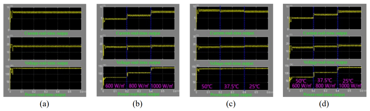
As shown in Fig. 12, the conductance increment method also achieves MPPT. Fig. 12(a) demonstrates that under conditions of [TeX:] $$25^{\circ} \mathrm{C}$$ temperature and 1,000 W/m² illumination intensity, the conductance increment method achieved maximum power tracking in a short period. Fig. 12(b) indicates that with a fixed environmental temperature, as the illumination intensity increased from 600 W/m² to 1,000 W/m², the output current significantly increased, whereas the increase in output voltage was not substantial, increasing output power. Fig. 12(c) shows that with constant environmental illumination intensity, as the environmental temperature decreased from [TeX:] $$50^{\circ} \mathrm{C} \text{ to } 25^{\circ} \mathrm{C}$$, output voltage increased and output current slightly decreased, increasing maximum power. Fig. 12(d) shows that when the environmental temperature decreased and illumination intensity increased simultaneously, the maximum output power of the PV cell increased.

In summary, after applying the conductance increment method to track the maximum power point of the PV cell, stability was maintained, and the accuracy was relatively high, which is consistent with the characteristics of this method.

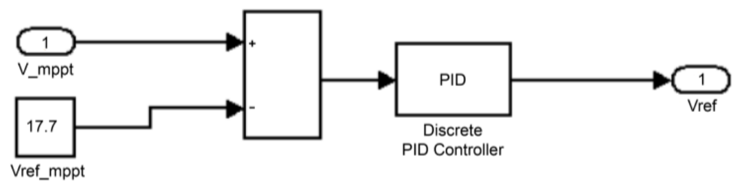
5.3 Simulation Analysis of Constant Voltage Method

The constant voltage MPPT algorithm module, as shown in Fig. 13, achieved MPPT by repeatedly comparing the calculated output voltage and input voltage at the specified maximum output power and then outputting the duty cycle through the algorithm. This duty cycle was determined by the PWM algorithm module shown in Fig. 11, which controls the Boost circuit to turn on or off, thereby tracking the maximum power point.

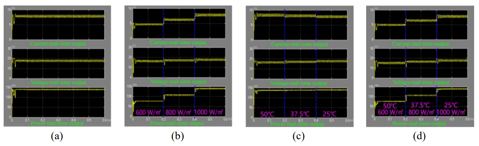
As shown in Fig. 14, the CVT effectively tracked the maximum power point. In Fig. 14(a), under conditions of [TeX:] $$25^{\circ} \mathrm{C}$$ temperature and 1,000 W/m2 units of irradiance, the CVT quickly achieved MPPT. In Fig. 14(b), with constant temperature and varying irradiance, the output current increased significantly as the irradiance decreased from 600 W/m² to 1,000 W/m², whereas the output voltage remained relatively stable, resulting in increased output power. From Fig. 14(c), when the ambient light intensity was constant, as the ambient temperature decreased from [TeX:] $$50^{\circ} \mathrm{C} \text{ to } 25^{\circ} \mathrm{C}$$, the output voltage, current, and maximum power change were insignificant. Fig. 14(d) illustrates the increase in maximum output power when the temperature decreased and irradiance increased simultaneously.

5.4 Comparison and Analysis of Simulation Results

First, based on the comparative analysis of the above simulation results, the correctness of the simulation module and its results can be determined. Second, by comparing the results of the three methods, compared to the CVT control method, the disturbance observation and conductance increment methods have a slower speed in tracking the maximum power point. Therefore, they are more suitable for PV power generation systems with slow changes in external environmental parameters. In situations where high speed is required for system power tracking, the CVT control method is suitable. Each method has advantages and disadvantages. In practical applications, an appropriate algorithm should be selected based on specific application requirements and external conditions to optimize the efficiency of the PV system.

6. Conclusion

Many methods can be used in the current research on MPPT technology, and each method has its strengths and limitations. Theoretical analysis and simulation results provide a reference for this. The limitations of the proposed method primarily include the trade-off between speed and efficiency, as the disturbance observation and conductance increment methods exhibit slower response times under rapidly changing environmental conditions. Additionally, the performance of existing methods under extreme weather conditions has not been thoroughly evaluated, and some high-performance control algorithms may introduce complexity and increase costs. Therefore, future research should focus on optimizing these algorithms to enhance tracking speed and accuracy, explore multivariable optimization strategies, and integrate smart control technologies, such as artificial intelligence. Furthermore, conducting long-term tests under various environmental conditions will help validate the effectiveness and reliability of these algorithms, ultimately improving the efficiency and adaptability of PV systems to meet future energy demands.

Conflict of Interest

The authors declare that they have no competing interests.

Funding

This project was funded by the 2024 Cost Research Project of State Grid Baiyin Power Supply Company (No. B72703241103); Shandong Provincial Natural Science Foundation (No. ZR2023MD086); and Shandong Province Science and Technology Small and Medium-Sized Enterprises Innovation Ability Enhancement Project (No. 2023TSGC0682).

References

- 1 A. Asnil, K. Krimadinata, E. Astrid, and I. Husnaini, "Enhanced incremental Conductance maximum power point tracking algorithm for photovoltaic system in variable conditions," Journal Européen des Systèmes Automatisés, vol. 57, no. 1, pp. 33-43, 2024. https://doi.org/10.18280/jesa.570104doi:[[[10.18280/jesa.570104]]]
- 2 A. M. Farayola, Y . Sun, and A. Ali, "Global maximum power point tracking and cell parameter extraction in photovoltaic systems using improved firefly algorithm," Energy Reports, vol. 8, pp. 162-186, 2022. https://doi.org/10.1016/j.egyr.2022.09.130doi:[[[10.1016/j.egyr.2022.09.130]]]
- 3 F. Bettahar, S. Abdeddaim, A. Betka, and C. Omar, "A comparative study of PSO, GWO, and HOA algorithms for maximum power point tracking in partially shaded photovoltaic systems," Power Electronics and Drives, vol. 9, no. 1, pp. 86-105, 2024. https://doi.org/10.2478/pead-2024-0006doi:[[[10.2478/pead-2024-0006]]]
- 4 V . Gali, B. C. Babu, R. B. Mutluri, M. Gupta, and S. K. Gupta, "Experimental investigation of Harris Hawk optimization‐based maximum power point tracking algorithm for photovoltaic system under partial shading conditions," Optimal Control Applications and Methods, vol. 44, no. 2, pp. 577-600, 2023. https://doi.org/ 10.1002/oca.2773doi:[[[10.1002/oca.2773]]]
- 5 J. Deng and Y . Wang, "Application of Lévy flight particle swarm optimisation in MPPT of photovoltaic system," International Journal of Electronics, vol. 111, no. 7, pp. 1143-1162, 2024. https://doi.org/10.1080/ 00207217.2023.2210305doi:[[[10.1080/00207217.2023.205]]]
- 6 B. Jie, P. Li, Y . Su, J. Su, and T. Liu, "Research on maximum power point tracking algorithm for photovoltaic arrays under partial shadow," Acta Energiae Solaris Sinica, vol. 44, no. 12, pp. 47-52, 2023. https://doi.org/ 10.19912/j.0254-0096.tynxb.2022-1363doi:[[[10.19912/j.0254-0096.tynxb.-1363]]]
- 7 R. Ding, "Maximum power point tracking method of photovoltaic system based on improved gray Wolf algorithm," Electronic Test, vol. 36, no. 22, pp. 47-50, 2022. https://doi.org/10.16520/j.cnki.1000-8519.2022. 22.026doi:[[[10.16520/j.cnki.1000-8519.2022.22.026]]]
- 8 M. Zhao, "Analysis and simulation of photovoltaic MPPT based on disturbance observation method," Electric Engineering, vol. 2022, no. 16, pp. 54-56+60, 2022. https://doi.org/10.19768/j.cnki.dgjs.2022.16.016doi:[[[10.19768/j.cnki.dgjs.2022.16.016]]]